 2022, Vol. 40
Institute of Oceanology, Chinese Academy of Sciences
Article Information
- YUN Tianyu, BU Xianhai, XING Zhe, LUAN Zhendong, FAN Miao, YANG Fanlin
- Automatic calibration for wobble errors in shallow water multibeam bathymetries
- Journal of Oceanology and Limnology, 40(5): 1937-1949
- http://dx.doi.org/10.1007/s00343-021-1283-7
Article History
- Received Sep. 3, 2021
- accepted in principle Oct. 23, 2021
- accepted for publication Nov. 24, 2021


2 National Marine Data and Information Service, Tianjin 300012, China;
3 Key Laboratory of Marine Geology and Environment & Center of Deep Sea Research, Institute of Oceanology, Chinese Academy of Sciences, Qingdao 266071, China;
4 Key Laboratory of Ocean Geomatics, Ministry of Natural Resources, Qingdao 266590, China
Multibeam echo sounding technology is one of the main approaches for seabed topography and geomorphology survey, with the characteristics of high precision, full coverage, and high efficiency (Hughes Clarke, 2000; Li et al., 2008). Due to the dynamic working environment of multibeam echo-sounder systems (MBES) and the characteristics of the multisensor combination of the system itself. The sounding results could be affected by various errors, including outliers caused by the system noise or ocean environmental noise, refraction errors caused by the incomplete surface sound velocity or sound velocity profile, tidal correction errors caused by imperfect tidal measurements or the inappropriate tidal calibration model, static draft errors of the transducer caused by the mass change of the carrier itself, dynamic draft errors caused by the uneven motion of the vessel, transducer installation errors and its calibration errors, nonconcentric array errors between sectors, and integration errors (Hare, 1995; Hare et al., 1995; Hughes Clarke, 2003a, b; Church, 2020). Except for the outliers, other errors can be divided into static errors and dynamic errors according to the nature of the measurement. The static errors are usually in larger magnitude and have received extensive attention. There are many mature methods to calibrate the static errors (Kammerer, 2000; Yang et al., 2013; Zhao et al., 2014; Hamilton et al., 2014; Guan et al., 2019; Bu et al., 2020). Compared with the static errors, the magnitude of the dynamic errors related to the motion sensor and the vessel motion is small, usually within the special order of standard in the International Hydrographic Organization (IHO) S-44 (IHO, 2008). The essence of wobble errors is the dynamic errors caused by the imperfect integration of motion sensors and transducers in MBES. When the magnitude of the dynamic errors is greater than 0.2% of the water depth (Maingot et al., 2019), the wobble errors may manifest as high frequency ribs or wobbles perpendicular to the heading direction in the high-precision shaded relief maps. The existence of wobble errors will affect the presentation of microtopography, thereby misleading the accurate analysis of seabed topography.
The problem of wobble errors in the MBES was firstly proposed by Hughes Clarke, Ocean Mapping Group (OMG) of New Brunswick University in Canada, and the error sources and manifestations of these errors are discussed in detail (Hughes Clarke, 2003b). Hughes Clarke realized the discrimination of these error sources based on the statistical method by analyzing correlations between motions and across-track profile-averaged residuals in the flat area. Inspired by Hughes Clarke's method, Yang et al.(2009, 2010) used wavelet analysis or Fourier transform to separate the high frequency wobble errors and the terrain trend. Then, a similar statistical method was used to locate errors. However, the above studies only focus on analyzing and discriminating single or dominant errors, ignoring the correlation between the errors, and do not give an effective method to eliminate these wobbles directly. To eliminate the errors existed in the motion sensor, Demkowicz et al. (2003) analyzed the influence of the roll error based on the simulated data and proposed to use the Kalman filter to correct wobbles in the bathymetries. Zhao et al. (2014) proposed a method of calibrating these errors based on the spectrum characters of seabed-topography trend and multibeam bathymetric data. Although the methods of Demkowicz and Zhao could iron these wobbles, the two methods are of strong subjective. When calibrating the installation errors of the transducers in the bathymetric data, Bjorke (2005) developed a method based on the soundings' georeferenced model. The installation parameters were solved by the least square algorithm, with the correlation between the parameters considered. Based on Bjorke's georeferenced model, Seube and Keyetieu (2017) and Keyetieu et al. (2018) realized the calibration of the multibeam installation errors and the motion time delay. However, the georeferenced model adopted by Bjorke ignored the independence of the transmitter and the receiver, which can lead to inherent errors in the bathymetric data and hinder the calibration results of these small wobble errors. Maingot's method considered the independence of the transmitter and the receiver, whereas the calibration process was complicated and the specific calibration model was not given (Maingot et al., 2019).
Consequently, limitations are as follows in the existed methods: 1) only useful for wobbles caused by single or dominant error; 2) lack of objective method considering the correlations between the errors; 3) lack of an accurate and efficient georeferenced model to eliminate these wobbles. To solve the problems above, this paper proposed a method calibrating the wobbles caused by single or multiple errors automatically. When constructing the georeferenced model, the independence between the transmitter and the receiver is considered, and the more simplified model is deduced specifically. Then, the wobble errors are considered as parameters in the improved georeferenced model to construct the calibration model. Finally, the genetic algorithm (GA) is used to search for the optimal error parameters with soundings in the flat area.
2 ANALYSIS OF ERROR SOURCES OF THE WOBBLESAs indicated in Maingot's study (Maingot et al., 2019), when the magnitude of wobble errors is greater than about 0.2% of the water depth, the high-frequency wobbles are easy to appear, as shown in Fig. 1. According to Hughes Clarke's study, the error sources can be divided into three types: 1) motion scale, time delay, and yaw misalignment; 2) X and Y lever arm errors; and 3) inaccurate surface sound speed correlated with vertical motion or rolling. Although the three kinds of errors all lead to wobbles, their manifestations are different in shallow water. The first type of error results in a linear tilting of the across-track profiles (Fig. 2a); the second type of error causes a linear lifting and falling of the across-track profiles (Fig. 2b); and the third type of error leads to a complex nonlinear tilting of the across-track profiles (Fig. 2c). Since the third type of error is related to the external factor out of the MBES, thus, this paper only focuses on addressing the first and second types of errors in the MBES.

|
| Fig.1 Shaded relief map with wobble errors (Hughes Clarke, 2003b) Reprinted with permission (Hughes Clarke, 2003b). Copyright 2003, International Hydrographic Review. |

|
| Fig.2 Three types of wobble manifestation (Hughes Clarke, 2003b) a. linear oscillation; b. linear heave; c. nonlinear oscillation. Reprinted with permission (Hughes Clarke, 2003b). Copyright 2003, International Hydrographic Review. |
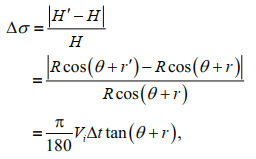
Due to serial port transmission or buffer setting, a certain time delay may exist between the motion sensor and the MBES. According to the research (Hughes Clarke, 2003b), it is found that the roll error caused by time delay Δt has the greatest influence on depth (Fig. 3). When time delay Δt exists, the depth error is defined by Eq.1.
 (1)
(1)

|
| Fig.3 Schematic diagram of depth distortion after introducing time delay or motion scale |
where Hʹ is the depth with time delay Δt, i.e., Hʹ=Rcos(θ+rʹ); rʹ is the roll with time delay Δt, i.e., rʹ=r+ViΔt; Vi is the instantaneous angular rate.
For instance, a typical wave period of 10 s with a roll amplitude of 3° may provide a maximum rate up to 0.019°/ms (Hughes Clarke, 2003b). Taking the edge beam with beam steering angle θ being 60° as an example, when r is 2°, a time delay as small as 3 ms may cause depth errors up to 0.2% of the water depth, thereby leading to wobbles.
2.2 Motion scale ΔρThe output value of the motion sensor is a factor associated with the motion time series, that is, the error is a scale with the real value (Hughes Clarke, 2003b). The larger the real value is, the greater the error is, and vice versa. The roll error caused by the motion scale Δρ also has the greatest influence on the depth (Fig. 3). When there is a motion scale Δρ, the depth error can be obtained by Eq.2.
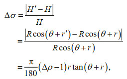 (2)
(2)where Hʹ is the depth with a motion scale Δρ, i.e., Hʹ=Rcos(θ+rʹ); rʹ is the roll with a motion scale Δρ, i.e., rʹ=Δρr.
For example, taking a general roll being 4°, Δρ as small as 1.014 will cause depth errors beyond 0.2% of the water depth in the edge area with steering angle θ beyond 60°, hence the wobbles are generated.
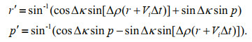
2.3 Yaw misalignment ΔκIdeally, the longitudinal axis (X-axis) of the motion sensor should be parallel to the longitudinal axis of the vessel to ensure that the measurements of the motion sensor can accurately reflect the motion of the vessel. However, due to imperfect manual installation, it is inevitable to introduce a certain angle bias Δκ (Fig. 4). According to the effect of yaw misalignment (Yang et al., 2010), the relationship between the actual vessel roll r, pitch p, and the sensor output roll rʹ, pitch pʹ can be calculated as Eq.3.

|
| Fig.4 Influence of yaw misalignment on the measured roll and pitch when the pitch of vessel exists (Yang et al., 2010) Reprinted with permission (Yang et al., 2010). Copyright 2010, Geomatics and Information Science of Wuhan University. |
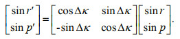 (3)
(3)For a general roll and pitch with the magnitude of 4° and 2°, respectively, yaw misalignment as small as 2° will cause depth errors beyond 0.2% of the water depth and lead to wobbles.
2.4 Lever arm errors [Δx, Δy]Lever arm errors are the offset errors of the motion sensor relative to the multibeam transducer. Since there is a certain offset between them, under the influence of the attitude, the transducer will produce an induced heave Hinduce. When errors exist in the lever arm, uncertainty will be introduced into the induced heave, which leads to the overall fluctuation of the swath. According to Hughes Clarke (2003b), lever arm errors in X and Y directions have a great influence, and the induced heave error caused by Δx and Δy lever arm errors can be calculated as Eq.4.
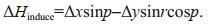 (4)
(4)For a general roll and pitch with the magnitude of 4° and 2°, respectively, both Δx and Δy as small as 1 m will cause the induced heave error up to 0.035 m. And these errors also will lead to wobbles when the water depth is approximately less than 17 m.
3 AUTOMATIC CALIBRATION METHOD OF WOBBLESSince Bjorke's georeferenced model does not consider the independence of the transmitter and the receiver, the accuracy of the model is low, which is unfavorable to the high-precision calibration of these small wobble errors. Therefore, this traditional model is improved firstly, and the calibration model coupled with these wobble error parameters is constructed based on the improved georeferenced model. Finally, the GA is used to search for the optimal error parameters.
3.1 Improvement of traditional georeferenced modelThe coordinate systems involved in the georeferenced model include the transducer coordinate system O-XtYtZt, the attitude coordinate system O-XmYmZm, the vessel coordinate system O-XvYvZv, and the local lever coordinate system O-NED (Yang et al., 2017). By using the sounding information of multibeam and measurements from each auxiliary sensor, the depth information under the multibeam transducer can be transformed to the geographical coordinate system based on a series of transformations, as shown in Fig. 5.

|
| Fig.5 Main coordinate systems in the MBES georeferenced model |
The IMU is generally located in the center of the vessel and the transducer is generally located on the side of the vessel or at the bottom of the vessel.
The coordinates of the soundings calculated based on the georeferenced model in the geographical coordinate system (Bjorke, 2005; Barnard, 2012) can be expressed as:
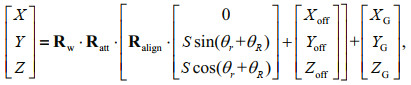 (5)
(5)where [0, Ssin(θr+θR), Scos(θr+θR)]T is the coordinates of the soundings in the transducer coordinate system; S is the oblique distance from the acoustic center of the transducer to the sounding, which can be obtained by ray tracing; θr is the received beam steering angle; θR is the sound ray refraction angle; [Xoff, Yoff, Zoff]T is the offset between the acoustic center of the transducer and the center of the global navigation satellite system (GNSS) antenna in the vessel coordinate system; [XG, YG, ZG]T is the geographical coordinates of the GNSS antenna center in Earth-Centered Earth-Fixed (ECEF) coordinate system; Rw is the rotation matrix consisted of the longitude and latitude (Wikipedia, 2021); Ratt and Ralign are the rotation matrices composed of the attitudes and installation angles, respectively; the rotation matrices of the angles in three directions are expressed as in Eq.6.
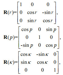 (6)
(6)where R(r), R(p), and R(κ) are the rotation matrices of roll (r), pitch (p), and yaw (κ), respectively.
In general, when multibeam transducers are installed, the transmitter is often parallel to the direction of the bow- and stern- line, while the receiver is perpendicular to the bow- and stern-line. According to the virtual concentric array (VCCA) method and beamforming theory (Beaudoin et al., 2004; Teng, 2012), the transmitted beam is more sensitive to the attitude of pitch rotation, while the received beam is more sensitive to the attitude of the roll rotation, as shown in Fig. 6.

|
| Fig.6 Influence of roll and pitch on the transmitted beam pattern and received beam pattern, respectively |
To derive the beam incidence vector (θ, Φ) considering the independence of the transmitter and the receiver, with the influence of the txsteer angle θt (Hamilton et al., 2014), the coordinate of the unit vector U=[0 0 1]T along the Z-axis in the transducer coordinate system is defined by Eq.7, whereas with the influence of the rxsteer angle θr (Hamilton et al., 2014) it is defined by Eq.8.
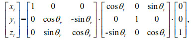 (7)
(7) (8)
(8)Comprehensively, with the combined influence of the txsteer angle θt and the rxsteer angle θr, the coordinate of the unit vector Uz in the transducer coordinate system is defined as follows:
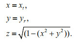 (9)
(9)Then, the beam incidence vector in the transducer coordinate system can be calculated by Eq.10.
 (10)
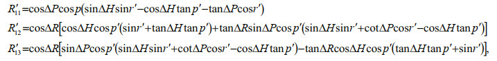
(10)Finally, by substituting Eq.10 into Eq.5, the improved georeferenced model for the soundings is given by Eq.11.
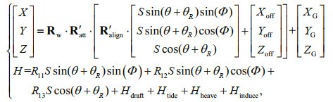 (11)
(11)where
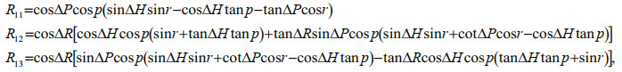
Rʹatt and Rʹalign are the rotation matrices composed of the attitudes and installation angles considering the independence of the transmitter and receiver, respectively; r is the roll at the receiving time; p is the pitch at the transmitted time; κ is the yaw at the transmitted time; ΔR is the roll installation angle of the receiver; ΔP is the pitch installation angle of the transmitter; ΔH is the yaw installation angle of the transmitter; Hdraft, Htide, Hheave, and Hinduce are the draft of the transducers, the tide, the heave, and the induced heave, respectively.
3.2 Calibration model coupled with wobble errorsAccording to Eq.3, when time delay Δt, motion scale Δρ, and yaw misalignment Δκ exist simultaneously, the output roll rʹ and pitch pʹ are given in Eq.12.
 (12)
(12)Since lever arm errors do not affect the angle, substituting Eqs.4 & 12 into Eq.11, the calibration model with the combined influence of the above four errors can be expressed in Eq.13.
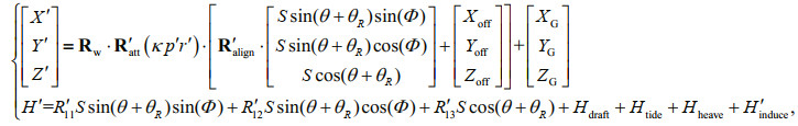 (13)
(13)where
H′induce is the induced heave with the influence of the above four errors.
3.3 Solving the error parametersThis paper proposes g(Δt, Δρ, Δκ, Δx, Δy) which represents the depth difference between the plane fitted by the least square method and the real-time estimated seabed. When the estimation of g(Δt, Δρ, Δκ, Δx, Δy) approaches zero, the corresponding parameter solution is the optimal solution. Typical seafloors, however, are not always planar. Fast changes in seafloor complexity, induced by the sudden appearance of such high frequency features, including sand waves, are likely unsuitable for analysis (Maingot et al., 2019). Therefore, to facilitate the elimination of wobble errors, flat areas are selected to avoid the influence of complex terrain changes on the performance of the proposed method. Since the wobble errors always manifest themselves as across-track ribbing, symmetrical soundings on both sides of the swath along the track are selected for the calibration.
Since g(Δ t, Δρ, Δκ, Δx, Δy) is difficult to linearize and solve by the least square method, the GA (Aytug et al., 2003; Goyal and Agrawal, 2013; FuRui et al., 2019) is used in this paper. The GA is proposed by Holland (1992), which can quickly search for the global optimal value. According to the principle of the GA, the fitness function is defined by Eq.14:
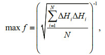 (14)
(14)where i is the serial number of soundings in the selected area; N is the number of soundings in the whole region.
The process of using the GA to automatically invert the best estimation of the corresponding error parameters can be divided into the following steps.
(1) Improving the georeferenced model;
(2) Introducing the corresponding error parameters into the improved georeferenced model;
(3) Calculating the coordinates of the soundings and fitting the plane;
(4) Encoding the feasible solutions of the corresponding error parameters by the real number;
(5) Using the random undirected initialization method to initialize the population in the corresponding error parameter range, according to the number of population set;
(6) Making each individual of the population evolve to generate new individuals, according to the set crossover probability and mutation probability (After testing, the crossover probability and mutation probability set in this paper are 0.5 which can not only ensure the optimal results but also ensure the computational efficiency.);
(7) Using the wheel selection method to calculate the probability of each individual being left, according to the fitness value of the new individual, and making the retained individuals form a new population;
(8) Repeating steps (6)–(7), if the set number of iterations is not reached or the optimal fitness value is less than the set threshold, or continuing step (9);
(9) Selecting the optimal individual which is the optimal solution of the corresponding error parameters, according to the fitness value. The specific process is shown in Fig. 7.

|
| Fig.7 Flow chart of the calibration method based on the GA |
Both simulated data and measured data are used to verify the proposed method. These datasets are preprocessed with noise removal, ray tracing, patch testing (Hughes Clarke, 2003b), and tide correction. In the simulated experiment, wobble errors are artificially introduced. In the experiment of measured data, the measured data with wobble errors are selected. Then, symmetrical soundings in the flat area on both sides of the swath along the swath are selected to construct the fitted plane and invert the wobble error parameters.
4.1 Simulated experimentThe data used for the simulated experiment are selected from the public dataset collected in Wellington Port, New Zealand in 2012 (Reson Company, 2012), which are acquired by Kongsberg EM2040. The average depth of the survey region is about 20.3 m. As described in Section 2, the common wobble problems are mainly caused by the motion scale, time delay, yaw misalignment, and X and Y lever arm errors. Therefore, the above wobble errors are taken as the representative for analysis. To verify the proposed method, these above wobble errors are artificially introduced and set to common values to get visible wobbles (Hughes Clarke, 2003b). The swath in the blue rectangle at the bottom of the survey region is used to analyze the results before and after calibration, as shown in Fig. 8.

|
| Fig.8 Survey region of simulated data |
In the original data, a 1.02 motion scale, 15-ms time delay, 2° yaw misalignment, and 1-m X and Y lever arm errors are introduced respectively. Then, the artificial errors are calibrated with the proposed method.
As shown in Fig. 9, under the influence of motion scale, time delay, and yaw misalignment, the edge of the swath has obvious wobbles (Fig. 9a, c, e). While the whole swath undulating phenomenon is introduced due to the X and Y lever arm errors (Fig. 9f). After calibration with the proposed method, the introduced wobble errors are eliminated. With our method, the final wobble error parameters of motion scale, time delay, yaw misalignment, and lever arm errors are approximately 1.018, 14.094 ms, 1.782°, 1.074 m, and 1.028 m, respectively, which are close to the originally introduced values.

|
| Fig.9 Illumination topographic maps before and after calibration of simulated data a. motion scale 1.02; b. calibrated results; c. time delay 15 ms; d. calibrated results; e. yaw misalignment 2°; f. calibrated results; g. lever arm errors 1 m; h. |
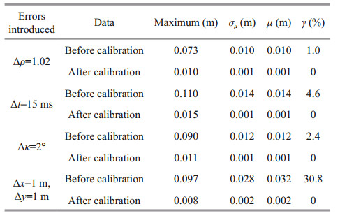
To verify the accuracy of our method, the histograms of depth differences between the original data and the calibrated data are shown in Fig. 10. After calibration, the distributions of depth differences are more concentrated near 0 under four situations. And indexes of the depth differences between the original data and data before and after calibration, such as the maximum absolute depth difference (maximum), the standard deviation (σμ), the mean depth difference (μ), and the percentage of soundings with depth error exceeding 0.2% of the water depth (γ) are calculated to evaluate the calibrated data. The results are shown in Table 1.

|
| Fig.10 Histograms of depth differences between original data and data before and after calibration under four situations a. motion scale 1.02; b. time delay 15 ms; c. yaw misalignment 2°; d. lever arm errors 1 m. |
|
As shown in Table 1, when a single error exists, the maximum absolute depth differences caused by 1.02 motion scale, 15-ms time delay, 2° yaw misalignment, and 1-m X and Y lever arm errors are 0.073, 0.110, 0.090, and 0.097 m, respectively, resulting in the depth error exceeding 0.2% of the water depth. After calibration, the maximum absolute depth differences are reduced to 0.010, 0.015, 0.011, and 0.008 m, respectively. The σμ and μ of the depth difference are reduced from centimeter level to millimeter level. Therefore, the accuracy is controlled to under 0.2% of the water depth.
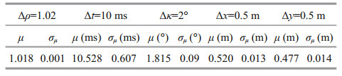
4.1.2 Multiple errorsIn this situation, a 1.02 motion scale, 10-ms time delay, 2° yaw misalignment, and 0.5-m X and Y lever arm errors are introduced to the original data at the same time. Then, the artificial errors are calibrated simultaneously.
Due to the coupling of these errors and the limited amount of data in the selected area, the calculated parameters have a certain uncertainty. To verify the stability of our method, the mean value (μ) and the standard deviation (σμ) of each error parameter after 10 times of automatic calculations are counted as shown in Table 2. The σμ of each error parameter is small. Therefore, our method has good stability and takes into account the coupling between error parameters. As shown in Fig. 11, under the influence of motion scale, time delay, yaw misalignment, and X and Y lever arm errors, the swath has obvious wobbles (Fig. 11a). After calibration with the proposed method, the introduced wobble errors are eliminated (Fig. 11b). As shown in Table 2, the mean values of motion scale, time delay, yaw misalignment, and lever arm error parameters are approximately 1.018, 10.528 ms, 1.815°, 0.520 m, and 0.477 m, respectively, which are close to the originally introduced values.

|
| Fig.11 Illumination topographic maps before and after calibration with four errors introduced a. results with four errors introduced; b. calibrated results. |
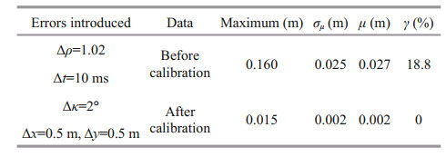
Then, the histograms of depth differences between original data and data before and after calibration in the case of four errors introduced are shown in Fig. 12. After calibration, the distributions of depth differences are more concentrated near 0. The indices of Maximum, σμ, μ, and γ are shown in Table 3.

|
| Fig.12 Histograms of depth differences between original data and data before and after calibration in the case of four errors introduced |
|
As shown in Table 3, when these four errors exist simultaneously, the maximum absolute depth difference caused by 1.02 motion scale, 10-ms time delay, 2° yaw misalignment, and 0.5-m X and Y lever arm errors is 0.160 m, resulting in the depth error exceeding 0.2% of the water depth. After calibration, the maximum absolute depth difference is reduced to 0.015 m, and the σμ and μ of the depth difference are reduced from 0.025 m and 0.027 m to 0.002 m, respectively. The accuracy of the calibrated data is within 0.2% of the water depth.
4.2 Experiment of measured dataThe measured data are provided by the Maps and Geospatial Products open platform of the National Oceanic and Atmospheric Administration (NOAA) and selected from the dataset collected in the Gulf of Mexico offshore, which are acquired by Simrad EM1002. The average depth of the survey region is about 179.8 m. These three swaths with wobble errors are selected to analyze the results before and after calibration. In the process of calibration, the motion scale, time delay, yaw misalignment, and lever arm errors are calculated at the same time because it is unknown whether each error exists.
The mean value (μ) and the standard deviation (σμ) of each error parameter after 10 times automatic calculations are counted as shown in Table 4. As shown in Fig. 13, the swaths have obvious wobbles (Fig. 13a). The wobble errors are eliminated after calibration with the proposed method (Fig. 13b). As shown in Table 4, the mean error parameters of motion scale, time delay, yaw misalignment, and lever arm errors by our method are approximately 1.003, 21.900 ms, 0.527°, 2.232 m, and 1.005 m, respectively. Therefore, it can be concluded that the wobbles in the swaths are mainly caused by the X and Y lever arm errors and time delay. The σμ of each error parameter is small, which shows that our method has good stability.


|
| Fig.13 Illumination topographic maps before and after calibration of measured data a. original measurements; b. calibrated results. |
Since the wobble errors always manifest themselves as across-track ribbing, the data before and after calibration are gridded to evaluate the calibrated data. The X-axis of the grid is perpendicular to the track, and the Y-axis is parallel to the track. The grid resolution is 28 m along the track and 7 m across the track, so the average number of soundings in each grid is about 8. The standard deviations of the depth in each grid are calculated before and after calibration, respectively. And the histograms of standard deviations of the depth are shown in Fig. 14.

|
| Fig.14 Histograms of standard deviations of the depth before and after calibration of measured data |
After calibration, the maximum standard deviation of the depth decreases from 0.729 m to 0.686 m, which is reduced by about 5.9%. The mean standard deviation of the depth decreases from 0.215 m to 0.191 m, which is reduced by about 11.2%. This further illustrates the effectiveness of our method.
5 DISCUSSION 5.1 Selection criterion for the flat terrainWhen choosing the flat terrain area to calibrate the wobbles, the absolute curvature of the seabed larger than 0.2°/m corresponds to gradual slopes (Mohammadloo et al., 2020). Thus, for a surface patch with curvature smaller than this threshold, a linear function can be used, otherwise, a bi-quadratic fit should be employed. However, this selection criterion for the flat terrain is complicated and time-consuming. In practice, the flat terrain is selected by visual inspection to construct the relatively fitted plane. The feasibility of the visual inspection method is also indicated by the significant calibrated results for both the simulated and the measured data in this paper.
5.2 Effect of the natural relief and roughnessThe data with high roughness, such as sand waves, and bedrock, seriously decrease the accuracy of the inverted results (Maingot et al., 2019). To verify the effect of the natural relief and roughness, the data in the red rectangle (Fig. 8) are selected to invert the corresponding parameters. Under this situation, the calibrated wobble error parameters of motion scale, time delay, yaw misalignment, and lever arm errors in the four cases are approximately 1.015, 15.168 ms, 4.968°, 1.472 m, and 1.342 m, respectively. The calibrated results are far from the originally introduced values. Thus, when the proposed method is used to calibrate wobble errors, data with protruding objects and high roughness should be avoided.
5.3 Limitations of the proposed methodAlthough our method can eliminate wobbles caused by the first and the second types of errors, for errors introduced by the third type of error, i.e., inaccurate surface sound speed correlated with vertical motion or rolling, the proposed method is not suitable. In addition, using a plane as the fitted surface also limits the general performance of our method. When facing a more complex seabed, the accuracy of our method will be affected. To improve the universality of our method the effectively fitted quadric surfaces (Hughes Clarke, 2003b; Maingot et al., 2019) can be used as constraints to improve our method.
6 CONCLUSIONThis paper focuses on the subtle wobble errors caused by the imperfect integration of motion sensors and transducers in shallow water multibeam bathymetries. To address the wobble errors in multibeam bathymetries, a precise calibration model associated with motion scale, time delay, yaw misalignment, and lever arm errors is constructed. And the GA is used to obtain the optimal values of these error parameters with soundings in the flat area. Experimental results showed that our method can effectively eliminate the wobbles caused by single or multiple wobble errors in shallow water areas, and the accuracy of the calibrated data is controlled within 0.2% of the water depth. The proposed method has significance in the precise calibration of dynamic errors in shallow water multibeam bathymetries.
7 DATA AVAILABILITY STATEMENTThe datasets generated during and/or analyzed during the current study are available from the corresponding author on reasonable request.
Aytug H, Khouja M, Vergara F E. 2003. Use of genetic algorithms to solve production and operations management problems: a review. International Journal of Production Research, 41(17): 3955-4009.
DOI:10.1080/00207540310001626319 |
Barnard T E. 2012. Geometrically derived ray-theory results and direct verification of the Pekeris solution for unbounded constant-gradient media. IEEE Journal of Oceanic Engineering, 37(2): 244-254.
DOI:10.1109/JOE.2012.2188161 |
Beaudoin J D, Hughes Clarke J E, Bartlett J E. 2004. Application of surface sound speed measurements in post-processing for multi-sector multibeam echosounders. International Hydrographic Review, 5(3): 17-32.
|
Bjorke J T. 2005. Computation of calibration parameters for multibeam echo sounders using the least squares method. IEEE Journal of Oceanic Engineering, 30(4): 818-831.
DOI:10.1109/JOE.2005.862138 |
Bu X H, Yang F L, Ma Y, et al. 2020. Simplified calibration method for multibeam footprint displacements due to non-concentric arrays. Ocean Engineering, 197: 106862.
DOI:10.1016/j.oceaneng.2019.106862 |
Church I W. 2020. Multibeam sonar ray-tracing uncertainty evaluation from a hydrodynamic model in a highly stratified estuary. Marine Geodesy, 43(4): 359-375.
DOI:10.1080/01490419.2020.1717695 |
Demkowicz J, Bikonis K, Stepnowski A, et al. 2003. Geocorrection and filtering of 3D bottom images from multi-beam sonar records. The Journal of the Acoustical Society of America, 114(4): 2346.
DOI:10.1121/1.4781123 |
FuRui, Al-Absi M A, Lee H J. 2019. Introduce a specific process of genetic algorithm through an example. In: Proceedings of 2019 International Conference on Information and Communication Technology Convergence. IEEE, Jeju, Korea (South). p. 422-425, https://doi.org/10.1109/ICTC46691.2019.8939728.
|
Goyal T, Agrawal A. 2013. Host scheduling algorithm using genetic algorithm in cloud computing environment. International Journal of Research in Engineering & Technology, 1(1): 7-12.
|
Guan M L, Li Q Q, Zhu J S, et al. 2019. A method of establishing an instantaneous water level model for tide correction. Ocean Engineering, 171: 324-331.
DOI:10.1016/j.oceaneng.2018.11.016 |
Hamilton T, Beaudoin J, Hughes Clarke J E. 2014. A more precise algorithm to account for non concentric multibeam array geometry. In: Proceedings of Canadian Hydrographic Conference 2014. The Canadian Hydrographic Association, St. John's N & L.
|
Hare R, Godin A, Mayer L. 1995. Accuracy Estimation of Canadian Swath (Multibeam) and Sweep (Multi-transducer) Sounding Systems, Internal Report. Canadian Hydrographic Service, Fredericton. p. 15-45.
|
Hare R. 1995. Depth and position error budgets for mulitbeam echosounding. International Hydrographic Review, 72(2): 37-69.
|
Holland J H. 1992. Adaptation in Natural and Artificial Systems: an Introductory Analysis with Applications to Biology, Control, and Artificial Intelligence. MIT Press, Cambridge, USA. 211p.
|
Hughes Clarke J E. 2000. Acoustic seabed surveying—meeting the new demands for accuracy, coverage and spatial resolution. Geomatica, 54(4): 473-485.
|
Hughes Clarke J E. 2003a. A reassessment of vessel coordinate systems: what is it that we are really aligning? In: Proceedings of US Hydrographic Conference 2003. The US Hydrographic Conference, Mississippi.
|
Hughes Clarke J E. 2003b. Dynamic motion residuals in swath sonar data: ironing out the creases. International Hydrographic Review, 4(1): 6-23.
|
IHO. 2008. IHO Standards for Hydrographic Surveys. International Hydrographic Organization, Monaco. 28p.
|
Kammerer E. 2000. A new method for the removal of refraction artifacts in multibeam echosounder systems. ProQuest Dissertations Publishing, Ann Arbor, USA. 191p.
|
Keyetieu R, Seube N, Djine V, et al. 2018. Multi-beam echo sounders-INS automatic latency calibration. Marine Geodesy, 41(5): 477-493.
DOI:10.1080/01490419.2018.1478349 |
Li H S, Yao B, Zhou T et al. 2008. Shallow water high resolution multi-beam echo sounder. In: Proceedings of OCEANS 2008-MTS/IEEE Kobe Techno-Ocean. IEEE, Kobe. p. 1-5, https://doi.org/10.1109/OCEANSKOBE.2008.4531081.
|
Maingot B, Hughes Clarke J E, Calder B R. 2019. High frequency motion residuals in multibeam data: identification and estimation. In: Proceedings of the U.S. Hydrographic Conference 2019. The Hydrographic Society of America, Biloxi.
|
Mohammadloo H T, Snellen M, Simons D G. 2020. Assessing the performance of the multi-beam echo-sounder bathymetric uncertainty prediction model. Applied Sciences, 10(13): 4671.
DOI:10.3390/app10134671 |
Reson Company. 2012. Raw Data. In: Proceedings of the 6th International Conference on High-Resolution Survey in Shallow Water. University of New Hampshire, New Zealand.
|
Seube N, Keyetieu R. 2017. Multibeam echo sounders-IMU automatic boresight calibration on natural surfaces. Marine Geodesy, 40(2-3): 172-186.
DOI:10.1080/01490419.2017.1310156 |
Teng Y T. 2012. Sector-specific Beam Pattern Compensation for Multi-sector and Multi-swath Multibeam Sonars. University of New Brunswick, Fredericton. 107p.
|
Wikipedia. 2021. Local Tangent Plane Coordinates. https://en.wikipedia.org/wiki/Local_tangent_plane_coordinates#Local_north,_east,_down_(NED)_coordinates. Accessed on 2021-11-10.
|
Yang F L, Bao J Y, Hu X S. 2017. Oceanic Surveying and Mapping. Wuhan University Press, Wuhan, China. p. 12-17. (in Chinese)
|
Yang F L, Li J B, Liu Z M, et al. 2013. Correction for depth biases to shallow water multibeam bathymetric data. China Ocean Engineering, 27(2): 245-254.
DOI:10.1007/s13344-013-0021-0 |
Yang F L, Li J B, Wu Z Y, et al. 2009. The methods of removing instantaneous attitude errors for multibeam bathymetry data. Acta Geodaetica et Cartographica Sinica, 38(5): 450-456.
(in Chinese with English abstract) DOI:10.3321/j.issn:1001-1595.2009.05.012 |
Yang F L, Lu X S, Li J B, et al. 2010. Correction of imperfect alignment of MRU for multibeam bathymetry data. Geomatics and Information Science of Wuhan University, 35(7): 816-820.
(in Chinese with English abstract) DOI:10.13203/j.whugis2010.07.005 |
Zhao J H, Yan J, Zhang H M, et al. 2014. A new method for weakening the combined effect of residual errors on multibeam bathymetric data. Marine Geophysical Research, 35(4): 379-394.
DOI:10.1007/s11001-014-9228-6 |