 2022, Vol. 40
Institute of Oceanology, Chinese Academy of Sciences
Article Information
- HAN Yuting, LI Yangang, XU Changsan, LIU Lei, ZHAO Yanling, LI Wenqing, SONG Xiangzhou
- Coastal buoy observation of air-sea net heat flux in the East China Sea in summer 2020
- Journal of Oceanology and Limnology, 40(3): 907-921
- http://dx.doi.org/10.1007/s00343-021-1012-2
Article History
- Received Jan. 29, 2021
- accepted in principle Apr. 25, 2021
- accepted for publication Jun. 15, 2021


2 National Marine Environmental Forecasting Center (NMEFC), Beijing 100081, China;
3 East China Sea Bureau of MNR, Shanghai 200081, China;
4 Institute of Oceanographic Instrumentation, Qilu University of Technology, Qingdao 266075, China;
5 The PLA 31010 Units, Beijing 100081, China
The heat fluxes at the air-sea interface include radiative fluxes and turbulent heat fluxes, which are fundamental physical processes for studies of upper ocean dynamics and air-sea interactions. The surface net heat flux (Qnet) is composed of mainly solar shortwave radiation (SW), longwave radiation (LW), evaporative latent heat flux (LH), and conductive sensible heat flux (SH). Qnet and surface wind stress are two main drivers of the evolution of the oceanic mixed layer (Price, 1979). In the tropical ocean, the evaporative LH associated with high sea surface temperature (SST) and significant evaporation primarily balances the incoming solar radiation (Carton and Zhou, 1997). The heat flux released from the warmest sea surface in the warm pool region (the western part of the tropical Pacific Ocean delineated by the 28-℃ isotherm of SST) drives atmospheric deep convection and affects the global atmospheric circulation (Bjerknes, 1969; Graham and Barnett, 1987). At high latitudes, when solar radiation is weak, the air-sea turbulent heat fluxes (LH+SH) determine the SST variations (Cayan, 1992) under air-sea feedback mechanisms (Frankignoul and Kestenare, 2002). Thus, producing accurate air-sea heat flux products is vital for understanding air-sea interactions.
However, the air-sea fluxes suffer from great biases over the global oceans among different heat flux products (Yu, 2019; Song, 2020a), especially in the western boundary current systems and at high latitudes (Fig.A1 in Song, 2020a). This bias impedes our accurate understanding of upper ocean processes and climate changes. The uncertainties of the heat fluxes are basically induced by different flux algorithms and essential air-sea variables for the flux calculations. Therefore, comparisons between pointto-point observations (e.g., buoy observations) and products are one of the effective ways to identify flux biases (Gleckler and Weare, 1997; Josey, 2001; Brunke et al., 2011), which helps further improve different heat flux products. Buoy observations can also provide reliable air-sea variables to validate the flux products, for example, the reanalysis and objectively analyzed products based on the available marine observations.
The East China Sea (ECS) is close to the Kuroshio, where the heat flux is released into the atmosphere and contributes to the global heat flux budget balance due to the significant air-sea differences in temperature and specific humidity (Kubota et al., 2008; Konda et al., 2010). However, the heat flux biases in this region are also larger than those in other regions (Song, 2020a). Full-flux observations in the ECS are rare, although some operational buoys have been deployed for marine disaster (for example, tropical cyclone) monitoring. The authors of this paper equipped operational buoys with radiative measurements to obtain the full flux in order to examine the uncertainties in flux products in the ECS. In addition, a recent study by Song and Yu (2017) showed that the air-sea heat fluxes in coastal regions play a non-negligible role in contributing to the basin-scale energy budget. With high-resolution modeling grids and accurate coastline data, the simulation of the mean heat flux in a semiclosed basin closely matches the ocean heat content because the land-sea processes can be captured well at synoptic scales. Figure 1 shows the evident gradients of SST and Qnet in ERA5, highlighting the importance of buoy observations in the ECS for the validation of air-sea processes. Relatively low Qnet values can be obtained off the Changjiang (Yangtze) River, while high Qnet values can be seen in the open ocean of the ECS. A significant Qnet difference of approximately 60 W/m2 occurs between these two areas.

|
| Fig.1 The mean Qnet=Qsw–Qlw–Qlh–Qsh (W/m2) from June to August 2020 in the northwestern Pacific based on the reanalysis of ERA5 The mean SST (℃) is shown by black contours with a contour interval of 1 ℃. The location of the buoy is marked by a purple solid dot off the Changjiang River. |
The new data in this study shed light on the magnitude of the summer Qnet in the ECS, which has rarely been measured. The three-month time series heat flux data from a specific location in the ECS provide a good chance to make a detailed assessment of reanalysis datasets, such as the 5th major atmospheric reanalysis produced by the European Centre for Medium-Range Weather Forecasts (ECMWF), which is called ERA5 for short (Hersbach et al., 2019, 2020), and the Modern-Era Retrospective analysis for Research and Applications, Version 2 (MERRA-2) (Gelaro et al., 2017).
We described the first full-flux observations in the ECS, with radiation observations from an operational 10-m buoy (Fig. 2) affiliated to and maintained by the State Oceanic Administration (SOA), Ministry of Natural Resources (MNR), China. Qnet was constructed in terms of radiative observations and turbulent heat fluxes based on the observed air-sea variables. The observed air-sea variables and heat fluxes were compared with the new reanalysis, helping find the biases in the reanalysis and enhances our confidence in using this product in this region. The remainder of this paper is organized as follows: Section 2 introduces the buoy observations and heat flux calculation algorithms, Sections 3.1 and 3.2 show the results of the observations of the full heat fluxes in summer and their variations associated with the air-sea variables, Section 3.3 provides the comparisons between the buoy observations and reanalysis and identifies the biases in the reanalysis, Section 4.1 discusses the reasons for the deviation, Section 4.2 assesses the overall simulation capability of the 4 reanalyzed products, and a summary is given in Section 5.

|
| Fig.2 Photographs of the buoy used in the East China Sea The left panel shows in-situ observations by the 10-m operational buoy in the ECS maintained by the East China Sea Bureau of the MNR. The observation height of the meteorological variables is approximately 11 m. The right panel shows an enlarged figure to show the meteorological sensors at the top of the buoy. |
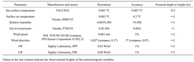
An air-sea 10-m buoy (Fig. 2) was deployed in the ECS at 122.4°E / 31.4°N, as indicated by the purple solid dot in Fig. 1. This buoy provided high-resolution observations of standard meteorological variables (detailed information in Table 1), including surface wind speed, wind direction, surface air temperature (SAT), SST, relative humidity (RH), and sea level pressure (SLP). The observational heights for wind, SAT, and RH were 11 m above the sea surface, while the sensors for measuring the SST were located at a depth of -0.5 m. The temporal resolution of the meteorological parameters and SST was 30 min. The daily mean variables were calculated by averaging the high-resolution measurements. Three months of data from June to August 2020 were used here to investigate the variations in air-sea heat fluxes in the ECS.
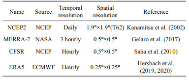
Four heat flux products were used in this study, including NCEP-DOE Reanalysis 2 (NCEP2) (Kanamitsu et al., 2002), MERRA-2, the NCEP Climate Forecast System Reanalysis (CFSR) (Saha et al., 2010), and ERA5. All the variables were constructed into daily means from June to August 2020. NCEP2 is the first generation of atmospheric reanalysis products and applies a zero surface balance constraint over the global ocean. NCEP2 uses a state-of-the-art analysis/forecast system to perform data assimilation using historical data from 1979 through the year before the current year. Three recently updated atmospheric reanalyses, namely, CFSR, ERA5, and MERRA-2, were also included in the analysis. Detailed information about the 4 reanalysis products is summarized in Table 2.
|
CFSR was initially completed over the 31-year period from 1979 to 2009. CFSR has created selected time series products at hourly temporal resolution by combining either 1) the analysis and one- through five-hour forecasts or 2) the one- through six-hour forecasts for each initialization time. After March 2011, the data from Climate Forecast System Version 2 (CFSv2) replaced CFSR. ERA5 is the fifthgeneration of ECMWF reanalysis for the global climate and weather for the past 4 to 7 decades. ERA5 replaces the ERA-Interim reanalysis. MERRA-2 data provide data from 1980 to present. This new global reanalysis replaces and extends the original MERRA dataset (Gelaro et al., 2017). MERRA-2 data are managed by the NASA Goddard Earth Sciences (GES) Data and Information Services Center (DISC). The high temporal resolution data from the reanalysis were constructed into daily mean values for comparisons with buoy observations in this study.
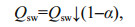
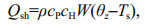
2.2 Air-sea flux calculation methodQnet consists of four components as follows:
 (1)
(1)where Qsw represents the net downward SW, Qlw represents the net upward LW, Qlh represents the LH (positive is upward), and Qsh represents the SH (positive is upward).
For buoy observation data:
 (2)
(2)where Qsw↓ denotes the incoming solar radiation directly measured by the buoy, and Qsw↑ denotes the upward shortwave radiation flux.
For NCEP2 and CFSR data:
 (3)
(3)where Qsw↓ denotes the downward shortwave radiation flux. Although the surface albedo α is not constant but changes with the surface state, the mean value is set to 0.06 according to the conventional choice for buoy observations (Fairall et al., 1996b).
For buoy observation data, the net LW (Qlw) is calculated from the upward LW (Qlw↑) associated with the surface thermal state and the observed downward LW (Qlw↓) (Dickey, 1994) as follows:
 (4)
(4)where Qlw↓ as observed directly by the buoy. The upward LW leaving the sea surface includes two parts (Eq.5): one is the emissions associated with SST (Fairall et al., 1996a, 2003; Alappattu et al., 2017), and the other part is the reflection of downward LW (Dickey, 1994):
 (5)
(5)where σ=5.7×10⁻⁸ is the Stefan-Boltzmann constant and εs=0.985 is the surface emissivity, which is associated with the temperature and wavelength. Ts denotes SST. In this study, the surface net LW is defined as the difference between the downward longwave radiation (DLW) associated with atmospheric absorption, emission, and scattering within the entire atmospheric column and the upward longwave radiation (ULW) emitted and reflected by the ocean surface (Eq.5).
Following Eq.4, Qlw↓ and Qlw↑ in NCEP2 and CFSR were both provided by the reanalysis data. Based on buoy observation data, turbulent heat fluxes, namely, LH and SH, are estimated by bulk formulas (Liu et al., 1979; Large and Pond, 1981; Clayson et al., 1996; Fairall et al., 1996b, 2003; Edson et al., 2013), following the Monin-Obukhov similarity theory (Monin and Obukhov, 1954):
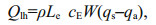 (6)
(6) (7)
(7)where qs≅0.98qsat(Ts) and θz≅Tz+γz.
In above equations, Qlh is LH, Qsh is SH, W is the wind speed, ρ is the density of air, Le is the latent heat of evaporation, and cP is the specific heat capacity of air. The turbulent exchange coefficients for LH and SH are denoted by cE and cH, respectively. The surface and near-surface atmospheric specific humidity are denoted by qs and qa, respectively. Ts is SST. qs is the saturation-specific humidity qsat of air at temperature Ts and includes a 2% reduction, which is caused by a typical salinity of 34. θz includes a correction for the adiabatic lapse rate γ. Tz is the air temperature at height z.
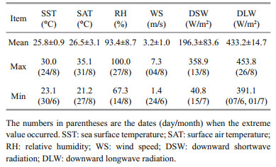
3 RESULT 3.1 Air-sea variables from buoy observations in summerFigure 3a shows that the daily mean SAT and SST in the summer in the ECS increased by approximately 7 ℃, and the increase was the most significant in August. In general (Table 3), SAT (26.5 ℃) is slightly higher than SST (25.8 ℃) in summer. SAT also fluctuated with higher magnitudes (3.1 ℃) than SST (0.9 ℃). As shown in Table 3, the daily mean summer SST in the ECS was 25.8 ℃, the highest temperature was 30.0 ℃ on August 24, and the lowest temperature was 23.1 ℃ on June 30. The average daily summer SAT of the ECS was 26.5 ℃, the highest SAT reached 35.1 ℃ on August 31, while the lowest was 21.2 ℃ on August 27 due to the potential effects from tropical cyclone Bavi. The variations in SAT and SST are caused by seasonal cycles.

|
| Fig.3 Time series of daily mean SST (blue, unit: ℃) and SAT (red, unit: ℃) (a), relative humidity (RH, unit: %) (b), wind speed (WS, unit: m/s) and wind direction (WD) (c) from June to August 2020 During the observational period, the measurements of SST and wind were not transmitted normally, thus the missing data were not used for calculation in this study. The red line in (c) represents the boundary where wind speed is zero. |
|
As shown in Fig. 3b, RH ranged from 80% to 100%, indicating that water vapor in the ECS was close to saturation and that the air was relatively humid in summer. Shown in Table 3, the average RH in the ECS region in summer was 93.4%, the highest RH was 100.0% on August 27, and the lowest RH was 67.3% on August 14. RH was high throughout the summer because water vapor in the ECS was humid and saturated in summer. In addition, RH can be affected by synoptic weather processes. Figure 3c shows that the southeasterly wind and the southerly wind prevail in summer, as was found in previous studies (Ding, 1994). The average wind speed was 3.2 m/s, the highest was 7.3 m/s on August 4, and the lowest was 1.4 m/s on June 24.
Figure 4 shows that downward shortwave radiation (DSW) presented an evident oscillation with a standard deviation (SD) of 83.6 W/m2 in the summer in the ECS. This oscillation may be caused by the cloud fraction associated with synoptic weather processes (Cess et al., 1995; Pilewskie and Valero, 1995; Ramanathan et al., 1995). The average value of DSW was 196.3 W/m2; however, the maximum value reached 358.9 W/m2 on August 13 and the minimum value was only 40.8 W/m2 on July 15. DSW showed a significant upward trend in August with the changing solar zenith angle in summer. Compared with DSW, DLW exhibited relatively weak variations, with an SD of 83.6 W/m2. The average DLW value was 433.2 W/m2, and the maximum value was 453.8 W/m2 on August 26, while the minimum value was 391.1 W/m2, which occurred on both June 7 and July 1, 2020. There was little difference in DLW in the three months in summer, with the minimum in August being slightly higher than the values in June and July. The extreme value of DLW in June and July coincided with that of SAT, which indicated that it was determined by SAT. However, in August, it showed no relation with SAT variations. A possible explanation may be associated with the cloud properties, whereas the buoy observations did not support such an examination, which was left for future studies.

|
| Fig.4 Time series of daily mean DSW (W/m2) (a) and DLW (b, W/m2) (b) from June to August 2020 DSW: downward shortwave radiation; DLW: downward longwave radiation. |
As shown in Fig. 5 and Table 4, the daily mean SW was the largest component among the four heat flux components with significant diurnal variations (approximately 500 W/m2 in amplitude, not shown here). The mean value was 183.2 W/m2. The daily mean SW showed large variation with an SD of 83.7 W/m2. The daily mean SW increased significantly in August, reaching 381.3 W/m2 on August 23, while the minimum value was 16.7 W/m2 on August 5. The amplitude of the daily mean LW oscillation in summer was also quite large, with an SD of 19.7 W/m2, and increases significantly in August, with an average of 26.5 W/m2. The maximum value reached 64.6 W/m2 on August 23, and the minimum value was -3.4 W/m2 on July 6. SW and LW were positive throughout the summer, and the magnitudes of SW were higher than those of LW, which means that the radiant heat flux was positive, meaning that the ocean obtains heat from the overlying atmosphere.

|
| Fig.5 The temporal evolution of the daily average SW (a), LW (b), SH (c), LH (d), and Qnet (e) from the ECS buoy from June to August 2020 Negative values of SW and Qnet represent the loss of heat from the ocean, and the positive values represent the opposite. Positive values of LW, SH, and LH represent the loss of heat from the ocean, and negative values represent the opposite. As the SST data were not transmitted normally during the observation period, the net LW, LH, and SH are absent at the beginning of June and end of August, although the downward SW and LW are fully observed. The dotted lines in (c–e) indicated that the value of SH, LH, Qnet is 0. |
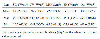
The mean values of SH and LH were both negative (SH, -1.5 W/m2; LH, -2.5 W/m2) and were of an order smaller than those of the radiant fluxes. The amplitude of LH was equivalent to LW, with an SD of 24.6 W/m2, while the amplitude of SH was the lowest of the four heat fluxes, with an SD of 5.3 W/m2. LH and SH both changed from positive to negative from June to August. Positive values of LH and SH represented the loss of heat from the ocean, while negative values represented the opposite. The ocean released heat in June and July because the SST (qs) is higher than the SAT (qa) when the atmospheric boundary condition was unstable. However, when the thermal state of the atmosphere was higher than that of the ocean in August, the boundary stability gradually stabilized, and the air-sea turbulent heat fluxes were directed from the atmosphere to the ocean. Therefore, the maximum value of LH reached 69.1 W/m2 on July 1, and the maximum value of SH reached 15.4 W/m2 on July 15. In August, both LH and SH had minimum values on August 4, which were -97.3 W/m2 for LH and -23.8 W/m2 for SH, indicating a loss of heat in the ocean.
During the whole observation period, the mean Qnet was 139.7 W/m2, which was mainly affected by SW, LW, and LH and showed an oscillating trend with an SD of 77.7 W/m2. The net SW was primarily balanced by LH and LW, while the role of the air-sea SH was secondary. Qnet increased significantly in July and August. Qnet reached a maximum value of 291.6 W/m2 on August 4, while the minimum value was -41.6 W/m2 on July 15. There was heavy rainfall (https://www.ecmwf.int/) on July 15, and thus, the SAT was associated with the lowest value of 23 ℃, which was 15 ℃ lower than the mean temperature of 38 ℃ in July. The SH due to rainfall-induced surface cooling (Gosnell et al., 1995; Cronin and McPhaden, 1997) was not estimated in this study due to the lack of direct precipitation observations. DSW reached the minimum value (40.8 W/m2) due to the cloud effect. Both SH and LH reached a second maximum (SH: 15.4 W/m2, LH: 44.3 W/m2), while DLW (423.6 W/m2) remained close to the mean value (433.2 W/m2). Therefore, the minimum Qnet value occurred on July 15.
3.3 Comparisons between the buoy observations and reanalysisDue to the lack of long-term observation data of sea-air flux in the ECS, we selected 4 reanalysis datasets (NCEP2, MERRA-2, CFSR, and ERA5) to compare with the observation data (OBS). This was the first full-flux observation activity for an operational coastal buoy system. The observations were used to identify the bias in the reanalysis in the ECS to satisfy the demands for studying long-term flux changes and increase the confidence in using these products. Figure 6 shows that the temporal evolution of the 4 reanalysis datasets of the five fluxes was basically consistent with that of OBS. The main difference was strongly affected by synoptic weather processes (Song, 2021). LH in NCEP2 showed a large discrepancy at the end of July with respect to the buoy observations and other recent updated reanalysis data (Fig. 6d). Table 5 listed the heat flux differences between the observations and reanalysis. The mean differences of the four components were less than 13 W/m2 except for LH (36–60 W/m2). As seen from the LH in the left panel of Fig. 6d, the signs of LH in the observation data and LH in the reanalysis data were basically opposite after mid-July, which was different from other heat flux components. Therefore, the correlation coefficient of LH in Fig. 7 was very low. In view of the analysis in Section 4.1, in addition to the effect of the algorithm and wind speed, RH may be an important reason for this difference. The daily mean values are compared to avoid the effects of diurnal variations in heat fluxes, in particular, the SW. Among the four heat flux components, the differences in SW and LH between the reanalysis data and OBS had SD values greater than 37 W/m2, which was larger than the values for the other flux components of approximately 15 W/m2.

|
| Fig.6 The difference in SW (a, f), LW (b, g), SH (c, h), LH (d, i), and Qnet (e, j) between the buoy data (left panel) and the 4 reanalysis datasets (right panel) (units: W/m2) Dashed lines indicated that the difference between the 4 reanalysis datasets and buoy data was 0. |

|

|
| Fig.7 Taylor diagram for Qnet (number 5) and contributing heat fluxes (SW (1), LW (2), SH (3), LH (4)) of the 4 reanalysis datasets Note that the correlation coefficients for the radial line denote the relationship between the OBS and reanalysis datasets. In addition, the normalized standard deviations (standard deviation of the reanalysis divided by that of the observations) are presented on the x- and y-axes. The points inside the dashed curved line (1) mean that reanalysis datasets have lower variability than the observations. |
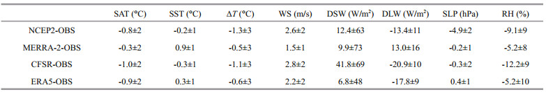
Table 5 shows that among all the differences between the reanalysis data and OBS of SW, the mean and SD of ERA5 were the lowest, while those of CFSR were the highest. As shown in Fig. 7, the SW of the ERA5 data was the closest to the OBS data in terms of the Taylor diagram (Taylor, 2001). The mean and SD of LW of NCEP2 were the lowest (3.0± 11 W/m2), and the means of CFSR and ERA5 were also low (CFSR: 5.0 W/m2, ERA5: 4.7 W/m2), while the mean of MERRA-2 was high (11.9 W/m2). However, the SDs of CFSR and ERA5 (CFSR: 18 W/m2, ERA5: 17 W/m2) were higher than that of MERRA-2 (12 W/m2). Figure 7 shows that the LW of the ERA5 data was also the closest to the OBS.
The mean and SD of SH of MERRA-2 were the lowest (3.9±6 W/m2), while the differences of the other three reanalysis data were not evident, with a mean and SD of approximately 10 W/m2. The mean and SD of the LH of the 4 reanalysis datasets were high, exceeding 36 W/m2. The mean Qnet of NCEP2 was the lowest, while the SD of ERA5 was the lowest, as shown in Fig. 7. Among the four flux components, the differences in SW and LW were relatively low, while those of LH and SH were relatively high. However, because the values of LH and SH are relatively small, the difference in Qnet was relatively small. Overall, the heat flux components in ERA-5 indicated a relatively improved ability to reproduce the observed heat fluxes among the 4 reanalysis products.
4 DISCUSSION 4.1 Causes of the difference between buoy data and reanalysis dataTo identify the error sources of the heat fluxes in the 4 reanalysis products, eight variables used for heat flux calculations are compared to observational parameters, including SAT, SST, ΔT(SST–SAT), wind speed, DSW, DLW, SLP, and RH. Table 6 shows that the differences in the 8 variables between the reanalysis data and the observed data were acceptable. Except for the individual variables of individual reanalysis products (e.g., DSW of CFSR), the mean value and SD of the differences were generally one or more orders lower than their own orders. All the reanalysis data indicate a cold and dry atmosphere with strong wind speed, which caused high air-sea temperature and humidity differences and high turbulent heat fluxes. In the reanalysis data, the colder atmosphere enhanced the air-sea temperature difference, and thus, the reanalysis products predicted a higher SH than the observations. Similarly, the drier atmosphere made the phase transition, such as vapor evaporation, stronger compared with the observation data. Combined with the enhanced wind speed, LH became significantly higher. Both of these were well illustrated in Fig. 6. The mean value and SD of the difference in wind speed were high compared with the order of 3.0 m/s, which was also reflected in Fig. 8. A high wind speed may be the reason why SH and LH had larger differences than the other flux components based on Eqs.6–7. Similar findings were also found in the reanalysis during the passages of tropical cyclones in a recent study by Song et al. (2021) using full-flux buoy observations in the southeastern Indian Ocean. Although the SW in all reanalysis products showed high estimates ranging from 9.9 to 43.3 W/m2 (Table 5), a relatively cold Qnet (-3.2 W/m2 to -51.2 W/m2) was obtained in Table 5 with high estimates of turbulent heat fluxes, in particular the LH (36.0 W/m2 to 59.5 W/m2). CFSR produced both a high SW due to the high DSW and a high LH due to a dry atmosphere. The net effect was a high Qnet due to the dominant role of a high SW in CFSR.

|
| Fig.8 Taylor diagram of eight observed elements for calculating fluxes and Taylor diagram of turbulent flux and recalculated turbulent flux a. the Taylor diagram for SAT (1), SST (2), ΔT (3), WS (4), DSW (5), DLW (6), SP (7), and RH (8) from 4 reanalysis datasets; b. the Taylor diagram for SH_R (recalculated SH based on bulk formulas using Eq.7, following the Monin-Obukhov similarity theory, ) (1), SH (2), LH_R (recalculated LH using Eqs. 6) (3), and LH (4) of 4 reanalysis datasets. |
The problems with small correlation coefficients reflected in the left panel of Fig. 8 mainly occur in SAT, wind speed (WS), and RH. The correlation of SAT was good in June and July until late August, when there was a tropical cyclone process. There was a large fluctuation in SAT observed by the buoys, but the reanalysis product did not reproduce it. This indicates the relatively poor ability of reanalysis to accurately reproduce synoptic weather scale processes. Although the variations in wind speed from reanalysis are in accordance with the OBS, the wind speed of reanalyzed products was consistently higher than that of OBS. The RH of the reanalyzed product was significantly different from the buoy data after late July. This could be due to the lower water vapor saturation in the reanalyzed products.
The exact magnitudes of the differences in DSW and DLW between the reanalysis and observations were summarized in Table 6. All the reanalysis products predict a high DSW ranging from 6.8 (ERA5) to 41.8 (CFSR) W/m2 with significant SDs. However, a low DLW has obtained for NCEP2 (-13.4 W/m2), CFSR (-20.9 W/m2), and ERA5 (-17.8 W/m2), while a high DLW was found for MERRA-2 at a magnitude of 13.0 W/m2.
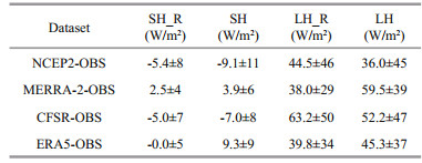
The flux component was related to not only the variables involved in the calculation but also the calculation method. In a recent study by Yu (2019), heat flux discrepancies were primarily induced by different heat flux algorithms, for example, different versions of bulk formulas. In this study, the LH and SH were recalculated using the output variables from the reanalysis, as shown in Table 7, using the same algorithm. The results indicate that by using the variables provided by the reanalysis data and the same method for calculating the flux from the buoy observation data, the SH and LH calculated by using the variables from the 4 reanalysis datasets were significantly improved compared with those from the direct model output (Table 7 and the right panel of Fig. 8).
It is still difficult to conclude which algorithm was more accurate in this study, except for the fact that the state of the atmosphere was colder and drier in the reanalysis products than in the in-situ observations. In addition, the direct observations of radiative fluxes provided a good test bed for the reanalysis. To calculate air-sea turbulent heat fluxes in the reanalysis, the old algorithm of the Louis scheme (Louis, 1979) was employed in ERA-5 and other operating forecast systems. The buoy-observed turbulent heat fluxes were based on bulk formulas, for example, COARE 3.0 (Coupled Ocean-Atmospheric Response Experiment) (Fairall et al., 1996b, 2003). There were significant differences between these schemes, which accounted for the discrepancies among the different reanalysis products.
4.2 Capability assessments of the 4 reanalysis dataBased on in-situ flux measurements, the mean fluxes of 4 reanalysis datasets (NCEP2, MERRA-2, CFSR, and ERA5) and buoy data were compared. Scatter plots reveal the assessment of the mean ability of the modeling/reanalysis simulation. Figure 9 shows that among the four components of air-sea flux, SW had the best simulation effect, while the LH simulation was poor due to a dry atmospheric environment, as presented above. LW and LH were higher than the buoy data, especially LH. A high LH resulted in a low Qnet. Furthermore, four reanalysis datasets were compared with the buoy dataset, which revealed that the difference in radiation flux was low, while the turbulent flux was high. To determine the mechanism for the uncertainties, the directly observed variables related to turbulent flux were analyzed, and the high wind speed was the main cause of this difference. Among all air-sea flux products, the air-sea flux in ERA5 was closer to the in-situ observations than the other products (Fig. 7). In addition, the spatial and temporal resolution of the reanalyzed product should also be one of the reasons for the difference between the reanalyzed products and the observed data. One of the reasons that ERA5 was closer to the OBS than the other reanalysis products is that not only its temporal resolution (hourly) is closest to the OBS (30 min) but also its spatial resolution (0.25°×0.25°) is the highest of the 4 reanalysis datasets (Table 2). Other researchers had also compared buoy data with reanalysis data in other areas of the ocean. For example, Song (2020b) compared the heat flux of buoy data with reanalysis products in the Bohai Sea and pointed out that the surface current, wind speed, unstable boundary conditions, and diurnal variation were the factors that caused the differences between the heat flux of the reanalysis product and the buoy data. Song (2020b) also concluded that MERRA-2 and ERA5 were superior to the OAFlux data in the Bohai Sea.

|
| Fig.9 Scatter diagrams of SW (a), LW (b), SH (c), LH (d), and Qnet (e) from the mean of the 4 reanalysis datasets (NCEP2, MERRA-2, CFSR, and ERA5) and the buoy dataset Dashed lines are diagonals, and solid lines are trend lines. The x-axis represents the buoy observations, and the y-axis denotes the mean magnitudes of the 4 reanalysis datasets. |
Air-sea heat flux is one of the frontier research areas in physical oceanography. Air-sea heat flux not only provides a thermal driving force for upper ocean dynamic processes but is also an important aspect of ocean-atmosphere interactions, which is a key factor in the study of climate change. However, there are still two problems in the current studies. One problem is how to more accurately quantify the heat flux under various ocean conditions to better understand the dynamic processes in the upper ocean. The second problem is how to deeply understand the mechanism of the changes in multiscale ocean-atmosphere dynamic processes affecting the air-sea heat flux to more accurately understand the ocean-atmosphere interaction process. Scientists have conducted more than half a century of research on the basic issue of the sea-air heat flux (Yu, 2019) and have a relatively clear level of understanding; for example, the spatial pattern of global distribution and the related principles of large-scale changes have been examined. However, because the physical mechanism has yet to be determined, the parameterization scheme must be improved; therefore, the global air-sea heat flux remains largely unknown and uncertain. In summary, there are still two questions in air-sea heat flux research, namely, "how much" and "how does it change". Currently, it is difficult to meet the needs of physical oceanography research, which demands heat flux precision within a magnitude of 10 W/m2 (Godfrey and Lindstrom, 1989). This study is only a starting point for full-flux observations in the ECS, where air-sea interactive processes are intense. In future works, the authors will continue to collect observations and improve the calculation algorithms, which will improve the understanding of the global heat flux balance and energy cycles.
5 CONCLUSIONIn this study, the full fluxes and associated air-sea variables based on operational buoy observations in the ECS in the summer of 2020 were provided and analyzed. This study revealed that the SAT was higher than the SST in summertime (which both exceed 25 ℃), the air was humid, the water vapor was almost saturated (93.4%), and southeasterly wind and southerly wind (3 m/s) prevail, as found in previous studies. The radiation flux was positive (SW, 183.2 W/m2, LW, 26.5 W/m2), the turbulent flux was negative (LH, -2.5 W/m2, SH, -1.5 W/m2), and the net heat flux was positive (139.7 W/m2), which represented heat gain by the ocean in summer. The time series of Qnet and other heat flux components were affected by synoptic weather processes. An important weather processed with heavy rainfall occurs on July 15, which was accompanied by high wind speed and high sea-air temperature differences. Therefore, a higher turbulent flux appeared at this time. However, cloud forcing caused low SW, and thus, the minimum Qnet value was obtained on that day. It should be noted that, the mean turbulent heat fluxes in summer were rather small due to the positiveto-negative switches in magnitudes. This was in close association with the marine boundary layer stability in the warm season. In summer, the SAT was higher than the SST, which generated a stabilized boundary condition and inhibited turbulent heat release from the ocean to the atmosphere.
It should be noted that, the mean turbulent heat fluxes in summer are rather small due to the positiveto-negative switches in magnitudes. This is in close association with the marine boundary layer stability in the warm season. In summer, as shown in Fig. 3, the SAT is higher than the SST, which generates a stabilized boundary condition and inhibits turbulent heat release from the ocean to the atmosphere. In addition, the turbulence flux of the reanalysis data is recalculated using the variables provided by the reanalysis data and the same method used to calculate the flux from the buoy observation data (Eqs.6–7). The SH and LH, which are recalculated, are significantly improved when compared with the direct model output. The old algorithm of the Louis scheme is employed for the reanalysis data, while bulk formulas are provided to calculate the buoy-observed turbulent heat fluxes. The significant differences between these methods can probably account for the discrepancies among different data (Yu, 2019). In future studies, the authors will focus on the validation of different heat flux algorithms.
The operational observations used in this study help identify the uncertainties in reanalysis and find better datasets for future studies in physical oceanography and air-sea interactions in the Northwest Pacific. In the next study, we will focus on the air-sea heat flux feedbacks on SST anomalies (Frankignoul et al., 1985, 1998; Frankignoul and Kestenare, 2002; Park et al., 2005; Hausmann et al., 2016) during post-El Niño summers with anticyclonic anomalies in the Northwest Pacific (Lau et al., 2000; Wang et al., 2000; Lu, 2001; Wang et al., 2003; Xie and Wang, 2020). In the summer of decaying El Niño phases, significant air-sea coupling processes and pronounced precipitation anomalies occur in the Northwest Pacific. Using the better reanalysis data (ERA5) based on this work, the mechanism of air-sea feedback in summer will be further explored under specific climate events (e.g., El Niño events). This study provides only the first step for understanding the basic aspects of air-sea coupled variability.
In order to meet the requirements for the long-term study of heat flux in the ECS, we compared 4 reanalysis datasets (NCEP2, MERRA-2, CFSR, and ERA5) with buoy data. Among the four components of air-sea flux of reanalysis datasets, SW had the best simulation effect, while the LH simulation was poor due to a drier and colder atmospheric environment of reanalysis datasets. LW and LH of reanalysis datasets were higher than the buoy data, especially LH. Among the 4 reanalysis datasets, the Qnet and four components of ERA5 were closer to the buoy data than other reanalysis datasets. In order to analyze the reasons for the difference of turbulent heat flux between the reanalysis datasets and buoy data, the turbulence flux of the reanalysis datasets was recalculated using the variables provided by the reanalysis data and the same method used to calculate the flux from the buoy observation data. The SH and LH, which were recalculated, were significantly improved when compared with the direct model output. The old algorithm of the Louis scheme was employed for the reanalysis data, while bulk formulas were provided to calculate the buoy-observed turbulent heat fluxes. The significant differences between these methods can probably accounted for the discrepancies among different data. The higher wind speed of the reanalysis products was another important reason for the difference. Although the analysis in this study was in one season, it was the first full-flux observation in this region. The operational observations used in this study could help identify the uncertainties in reanalysis and find better datasets for future studies in physical oceanography and air-sea interactions in the Northwest Pacific.
6 DATA AVAILABILITY STATEMENTThe datasets generated and/or analyzed during the current study are available from the corresponding author upon reasonable request.
7 ACKNOWLEDGMENTThe authors thank the joint cruise team from the East China Sea Bureau of Ministry of Natural Resources, China. The NECP2, MERRA-2, CFSR, and ERA5 data were downloaded from https://psl.noaa.gov, https://gmao.gsfc.nasa.gov, https://rda.ucar.edu, and https://www.ecmwf.int/, respectively. The authors appreciate the constructive comments and suggestions from the anonymous reviewers.
Alappattu D P, Wang Q, Yamaguchi R, Lind R J, Reynolds M, Christman A J. 2017. Warm layer and cool skin corrections for bulk water temperature measurements for air-sea interaction studies. Journal of Geophysical Research: Oceans, 122(8): 6470-6481.
DOI:10.1002/2017JC012688 |
Bjerknes J. 1969. Atmospheric teleconnections from the equatorial pacific. Monthly Weather Review, 97(3): 163-172.
DOI:10.1175/1520-0493(1969)097<0163:ATFTEP>2.3.CO;2 |
Brunke M A, Wang Z, Zeng X B, Bosilovich M, Shie C L. 2011. An assessment of the uncertainties in ocean surface turbulent fluxes in 11 reanalysis, satellite-derived, and combined global datasets. Journal of Climate, 24(21): 5469-5493.
DOI:10.1175/2011JCLI4223.1 |
Carton J A, Zhou Z X. 1997. Annual cycle of sea surface temperature in the tropical Atlantic Ocean. Journal of Geophysical Research: Oceans, 102(C13): 27813-27824.
DOI:10.1029/97JC02197 |
Cayan D R. 1992. Latent and sensible heat flux anomalies over the northern oceans: the connection to monthly atmospheric circulation. Journal of Climate, 5(4): 354-369.
DOI:10.1175/1520-0442(1992)005<0354:LASHFA>2.0.CO;2 |
Cess R D, Zhang M H, Minnis P, Corsetti L, Dutton E G, Forgan B W, Garber D P, Gates W L, Hack J J, Harrison E F, Jing X, Kiehi J T, Long C N, Morcrette J J, Potter G L, Ramanathan V, Ramanathan V, Subasilar B, Whitlock C H, Young D F, Zhou Y. 1995. Absorption of solar radiation by clouds: observations versus models. Science, 267(5197): 496-499.
DOI:10.1126/science.267.5197.496 |
Clayson C A, Fairall C W, Curry J A. 1996. Evaluation of turbulent fluxes at the ocean surface using surface renewal theory. Journal of Geophysical Research: Oceans, 101(C12): 28503-28513.
DOI:10.1029/96JC02023 |
Cronin M F, McPhaden M J. 1997. The upper ocean heat balance in the western equatorial Pacific warm pool during September-December 1992. Journal of Geophysical Research: Oceans, 102(C4): 8533-8553.
DOI:10.1029/97JC00020 |
Dickey T D, Manov D V, Weller R A, Siegel D A. 1994. Determination of longwave heat flux at the air-sea interface using measurements from buoy platforms. Journal of Atmospheric and Oceanic Technology, 11(4): 1057-1078.
DOI:10.1175/1520-0426(1994)011<1057:DOLHFA>2.0.CO;2 |
Ding Y H. 1994. Monsoons over China. Advances in Atmospheric Sciences, 11(2): 252.
DOI:10.1007/BF02682559 |
Edson J B, Jampana V, Weller R, Bigorre S, Plueddemann A, Fairall C, Miller S, Mahrt L, Vickers D, Hersbach H. 2013. On the exchange of momentum over the open ocean. Journal of Physical Oceanography, 43(8): 1589-1610.
DOI:10.1175/JPO-D-12-0173.1 |
Fairall C W, Bradley E F, Godfrey J S, Wick G A, Edson J B, Young G S. 1996a. Cool-skin and warm-layer effects on sea surface temperature. Journal of Geophysical Research: Oceans, 101(C1): 1295-1308.
DOI:10.1029/95JC03190 |
Fairall C W, Bradley E F, Hare J E, Grachev A A, Edson J B. 2003. Bulk parameterization of air-sea fluxes: updates and verification for the COARE algorithm. Journal of Climate, 16(4): 571-591.
DOI:10.1175/1520-0442(2003)016<0571:BPOASF>2.0.CO;2 |
Fairall C W, Bradley E F, Rogers D P, Edson J B, Young G S. 1996b. Bulk parameterization of air-sea fluxes for Tropical Ocean-Global Atmosphere Coupled-Ocean Atmosphere Response Experiment. Journal of Geophysical Research: Oceans, 101(C2): 3747-3764.
DOI:10.1029/95JC03205 |
Frankignoul C. 1985. Sea surface temperature anomalies, planetary waves, and air-sea feedback in the middle latitudes. Reviews of Geophysics, 23(4): 357-390.
DOI:10.1029/RG023i004p00357 |
Frankignoul C, Czaja A, L'Heveder B. 1998. Air-sea feedback in the North Atlantic and surface boundary conditions for ocean models. Journal of Climate, 11(9): 2310-2324.
DOI:10.1175/1520-0442(1998)011<2310:ASFITN>2.0.CO;2 |
Frankignoul C, Kestenare E. 2002. The surface heat flux feedback. Part Ⅰ: estimates from observations in the Atlantic and the North Pacific. Climate Dynamics, 19(8): 633-647.
DOI:10.1007/s00382-002-0252-x |
Gelaro R, McCarty W, Suarez M J, Todling R, Molod A, Takacs L, Randles C, Darmenov A, Bosilovich M G, Reichle R, Wargan K, Coy L, Cullathe R, Draper C, Akella S, Buchard V, Conaty A, Da Silva A, Gu W, Kim G K, Koster R, Lucchesi R, Merkova D, Nielsen J E, Partyka G, Pawson S, Putman W, Rienecker M, Schubert S D, Sienkiewicz M, Zhao B. 2017. The modern-era retrospective analysis for research and applications, version 2 (MERRA-2). Journal of Climate, 30(14): 5419-5454.
DOI:10.1175/JCLI-D-16-0758.1 |
Gleckler P J, Weare B C. 1997. Uncertainties in global ocean surface heat flux climatologies derived from ship observations. Journal of Climate, 10(11): 2764-2781.
DOI:10.1175/1520-0442(1997)010<2764:UIGOSH>2.0.CO;2 |
Godfrey J S, Lindstrom E J. 1989. The heat budget of the equatorial western Pacific surface mixed layer. Journal of Geophysical Research: Oceans, 94(C6): 8007-8017.
DOI:10.1029/JC094iC06p08007 |
Gosnell R, Fairall C W, Webster P J. 1995. The sensible heat of rainfall in the tropical ocean. Journal of Geophysical Research: Oceans, 100(C9): 18437-18442.
DOI:10.1029/95JC01833 |
Graham N E, Barnett T P. 1987. Sea surface temperature, surface wind divergence, and convection over tropical oceans. Science, 238(4827): 657-659.
DOI:10.1126/science.238.4827.657 |
Hersbach H, Bell B, Berrisford P, Hirahara S, Horányi A, Muñoz-Sabater J, Nicolas J, Peubey C, Radu Schepers D, Simmons Soci C, Abdalla S, Abellan X, Balsamo G, Bechtold P, Biavati G, Bidlot J, Bonavita M, De Chiara G, Dahlgren D, Dee D, Diamantakis M, Dragani R, Flemming J, Forbes R, Fuentes M, Geer A, Haimberger L, Healy S, Hogan R J, Hólm E, Janisková M, Keeley S, Laloyaux P, Lopez P, Lupu C, Radnoti G, De Rosnay P, Rozum I, Vamborg F, Villaume S, Thépaut J N. 2020. The ERA5 global reanalysis. Quarterly Journal of the Royal Meteorological Society, 146(730): 1999-2049.
DOI:10.1002/qj.3803 |
Hersbach H, Bell W, Berrisford P, Horányi A J M S, Nicolas J, Radu R, Schepers D, Simmons A, Soci C, Dee D. 2019. Global reanalysis: goodbye ERA-Interim, hello ERA5. Meteorology Section of ECMWF Newsletter, 159: 17-24.
DOI:10.1175/JCLI-D-16-0758.1 |
Josey S A. 2001. A comparison of ECMWF, NCEP-NCAR, and SOC surface heat fluxes with moored buoy measurements in the subduction region of the Northeast Atlantic. Journal of Climate, 14(8): 1780-1789.
DOI:10.1175/1520-0442(2001)014<1780:ACOENN>2.0.CO;2 |
Kanamitsu M, Ebisuzaki W, Woollen J, Yang S K, Hnilo J J, Fiorino M, Potter G L. 2002. NCEP-DOE AMIP Ⅱ Reanalysis (R-2). Bulletin of the American Meteorological Society, 83: 1631-1643.
DOI:10.1175/BAMS-83-11-1631 |
Konda M, Ichikawa H, Tomita H, Cronin M F. 2010. Surface heat flux variations across the Kuroshio extension as observed by surface flux buoys. Journal of Climate, 23(19): 5206-5221.
DOI:10.1175/2020JCLI3391.1 |
Kubota M, Iwabe N, Cronin M F, Tomita H. 2008. Surface heat fluxes from the NCEP/NCAR and NCEP/DOE reanalyses at the Kuroshio Extension Observatory buoy site. Journal of Geophysical Research: Oceans, 113(C2): C02009.
DOI:10.1029/2007JC004338 |
Large W G, Pond S. 1981. Open ocean momentum flux measurements in moderate to strong winds. Journal of Physical Oceanography, 11: 324-336.
DOI:10.1175/1520-0485(1981)011<0324:OOMFMI>2.0.CO;2 |
Lau K M, Kim K M, Yang S. 2000. Dynamical and boundary forcing characteristics of regional components of the Asian summer monsoon. Journal of Climate, 13(14): 2461-2482.
DOI:10.1175/1520-0442(2000)013<2461:DABFCO>2.0.CO;2 |
Liu W T, Katsaros K B, Businger J A. 1979. Bulk parameterization of air-sea exchanges of heat and water vapor including the molecular constraints at the interface. Journal of Atmospheric Sciences, 36(9): 1722-1735.
DOI:10.1175/1520-0469(1979)036<1722:BPOASE>2.0.CO;2 |
Louis J F. 1979. A parametric model of vertical eddy fluxes in the atmosphere. Boundary-Layer Meteorology, 17(2): 187-202.
DOI:10.1007/BF00117978 |
Lu R Y. 2001. Interannual variability of the summertime North Pacific subtropical high and its relation to atmospheric convection over the warm pool. Journal of the Meteorological Society of Japan, 79(3): 771-783.
DOI:10.2151/jmsj.79.771 |
Monin A, Obukhov A. 1954. Basic Laws of Turbulent Mixing in the Surface Layer of the Atmosphere. Tr. Akad. Nauk SSSR Geophiz,, 24(151): 163-187.
|
Pilewskie P, Valero F P J. 1995. Direct observations of excess solar absorption by clouds. Science, 267(5204): 1626-1629.
DOI:10.1126/science.267.5204.1626 |
Price J F. 1979. Observations of a rain-formed mixed layer. Journal of Physical Oceanography, 9(3): 643-649.
DOI:10.1175/1520-0485(1979)009<0643:OOARFM>2.0.CO;2 |
Ramanathan V, Subasilar B, Zhang G J, Conant W, Cess R D, Kiehi J T, Grassi H, Shi L. 1995. Warm pool heat budget and shortwave cloud forcing: a missing physics?. Science, 267(5197): 499-503.
DOI:10.1126/science.267.5197.499 |
Saha S, Moorthi S, Pan H L, Wu X, Wang J, Nadiga S, Tripp P, Kistler P, Woollen J, Behringer D, Liu H, Stokes D, Grumbine R, Gayno G, Wang J, Hou Y T, Chuang H Y, Juang H M, Sela J, Iredell M, Treadon R, Kleist D, Delst P V, Keyser D, Derber J, Ek M, Meng J, We H, Yang R, Lord S, Dool H V D, Kumar A, Wang W, Long C, Cheliah M, Xue Y, Huang B, Schemm J K, Ebisuzaki W, Lin R, Xie P, Chen M, Zhou S, Higgins W, Zou C Z, Liu Q, Chen Y, Han Y, Cucurull L, Reynolds R W, Rutledge G, Goldberg M. 2010. The NCEP Climate Forecast System Reanalysis. Bulletin of American Meteorological Society, 91: 1015-1057.
DOI:10.1175/2010BAMS3001.1 |
Song X Z, Ning C L, Duan Y L, Wang H W, Li C, Yang Y, Liu J J, Yu W D. 2021. Observed extreme air-sea heat flux variations during three tropical cyclones in the tropical southeastern Indian Ocean. Journal of Climate, 34(9): 3683-3705.
DOI:10.1175/JCLI-D-20-0419.1 |
Song X Z, Yu L S. 2017. Air-sea heat flux climatologies in the Mediterranean Sea: surface energy balance and its consistency with ocean heat storage. Journal of Geophysical Research: Oceans, 122(5): 4068-4087.
DOI:10.1002/2016JC012254 |
Song X Z. 2020a. Explaining the zonal asymmetry in the air-sea net heat flux climatology over the Antarctic circumpolar current. Journal of Geophysical Research: Oceans, 125(6): e2020JC016215.
DOI:10.1029/2020JC016215 |
Song X Z. 2020b. The importance of relative wind speed in estimating air-sea turbulent heat fluxes in bulk formulas: examples in the Bohai Sea. Journal of Atmospheric and Oceanic Technology, 37(4): 589-603.
DOI:10.1175/JTECH-D-19-0091.1 |
Song X Z. 2021. The importance of including sea surface current when estimating air-sea turbulent heat fluxes and wind stress in the Gulf Stream region. Journal of Atmospheric and Oceanic Technology, 38(1): 119-138.
DOI:10.1175/JTECH-D-20-0094.1 |
Taylor K E. 2001. Summarizing multiple aspects of model performance in a single diagram. Journal of Geophysical Research: Atmospheres, 106(D7): 7183-7192.
DOI:10.1029/2000JD900719 |
Wang B, Wu R G, Fu X H. 2000. Pacific–East Asian teleconnection: how does ENSO affect East Asian climate?. Journal of Climate, 13(9): 1517-1536.
DOI:10.1175/1520-0442(2000)013<1517:PEATHD>2.0.CO;2 |
Wang B, Wu R G, Li T. 2003. Atmosphere-warm ocean interaction and its impacts on Asian-Australian monsoon variation. Journal of Climate, 16(8): 1195-1211.
DOI:10.1175/1520-0442(2003)16<1195:AOIAII>2.0.CO;2 |
Xie M M, Wang C Z. 2020. Decadal variability of the anticyclone in the western North Pacific. Journal of Climate, 33(20): 9031-9043.
DOI:10.1175/JCLI-D-20-0008.1 |
Yu L S. 2019. Global air-sea fluxes of heat, fresh water, and momentum: energy budget closure and unanswered questions. Annual Review of Marine Science, 11: 227-248.
DOI:10.1146/annurev-marine-010816-060704 |