 2021, Vol. 39
Institute of Oceanology, Chinese Academy of Sciences
Article Information
- Shahanul ISLAM M., SUN Jun, LIU Haijiao, ZHANG Guicheng
- Environmental influence on transparent exopolymer particles and the associated carbon distribution across northern South China Sea
- Journal of Oceanology and Limnology, 39(4): 1430-1446
- http://dx.doi.org/10.1007/s00343-020-0236-x
Article History
- Received Jun. 8, 2020
- accepted in principle Aug. 3, 2020
- accepted for publication Oct. 5, 2020


2 Research Centre for Indian Ocean Ecosystem, Tianjin University of Science and Technology, Tianjin 300457, China;
3 Tianjin Key Laboratory of Marine Resources and Chemistry, Tianjin University of Science and Technology, Tianjin 300457, China
The South China Sea (SCS), especially its north (nSCS) is one of the productive zones among coastal seas of China (Liu et al., 2016). It is decorated with a number of dynamic features, which act as controlling factors on its ecosystem (Sun et al., 2012). Geodynamics of SCS showed the presence of rifted basin of continental shelf near these estuaries (Sibuet et al., 2016). Complex geophysical interactions driven by SCS summer monsoon (SCSSM) were observed in here which affect regional gyre dilution and temperature (Choi et al., 2016) near the Kuroshio (Tian and Wang, 2010). Additionally, ENSO wind driven SCS weather was observed during summer, controlled by western Pacific currents and wind circulations (Mao and Chan, 2005; Ding et al., 2018).It is also loaded by sediment and organic carbon (Jiao et al., 2018) through Modaomen, Lingdingyang, and Huangmaohai sub-estuaries. Among them, Lingdingyang or Zhujiang (Pearl) River estuary contribute most i.e. 0.1%–0.2% of total organic carbon carried by river in the world (Ni et al., 2008). Phytoplankton played an important role in this ecosystem i.e. carbon exchange, primary productivity, and so on (Sun et al., 2012). Its concentration, distribution, and associated particle transports were predicted to be highly influenced by these environmental factors and geophysical circulations as well (Xie et al., 2003; Yang et al., 2013; Huangfu et al., 2018).
Transparent exopolymer particles (TEP) are found as microgels through all aquatic systems in various sizes (Passow, 2002). They are formed by certain colloidal polysaccharide secretion from phytoplankton and bacteria (Alldredge et al., 1993). Theoretically, they are consumed and utilized by nekton (Miller et al., 2013), micronekton, zooplankton (Mari et al., 2017), and bacteria during its sinking process (Passow, 2002). Their formations influence vertical mass fluxes, restrict optical properties, and drive the basic carbon cycling in ocean (Mari et al., 2017). Additionally, primary and secondary production may have an indirect effect on TEP concentration, which may regulate global climate changes effectively (Wurl et al., 2011). On this note, interactions of TEP with environmental controlling factors need to be addressed more to understand their biogenic importance deeply.
Present study is focused on TEP distribution at nSCS and its probable contribution in carbon concentration across this transect. Notably, concentration of TEP has closer relation with the abundance of its primary source, phytoplankton (Passow et al., 1994) and showed positive correspondence with chlorophyll a (chl a) on a global scale (Passow, 2002). Alternatively, coagulation of dissolve organic matter (DOM) by abiotic process is also a source of the TEP (Chin et al., 1998). It generates colloidal organic matter, especially at surface of ocean (Passow and Alldredge, 1994; Passow, 2000). Besides, it was reported that TEP increased from the bottom of the mixed layer depth (MLD) to the top of the subsurface chlorophyll maximum (SCM) based on active photosynthesis (Kodama et al., 2014). Though nSCS is a eutrophic zone with all these factors (Huangfu et al., 2018), no studies were done on TEP distributions and its contributions. Therefore, it will be worthy to investigate the influence of environmental factors on TEP at nSCS. Furthermore, production of TEP also influenced by water turbulence, laminar shear and Brownian motion (Passow, 2000; Burd and Jackson, 2009), which are notable features of nSCS (Choi et al., 2016).
Positive floating mechanism of TEP can drive it to accumulate at the sea surface microlayer (Wurl et al., 2009) and provide gelatinous composition to this interfacial film between atmosphere and ocean surface (Wurl and Holmes, 2008). Measuring vertical distribution of TEP has been done in different seas (Bar-Zeev et al., 2009; Ortega-Retuerta et al., 2010; Bar-Zeev et al., 2011) and oceans (Wurl et al., 2011). In estuaries, TEP sedimentation measurement near East China Sea (Changjiang (Yangtze) River estuary) and TEP aggregation near SCS (Zhujiang River estuary) were examined previously (Sun et al., 2010; Guo and Sun, 2018). However, there is no sufficient reports on deep sea profiling of TEP and its distribution, especially at the nSCS. Comparison of TEP between on-shelf and the open SCS areas were insufficient too. Therefore, the present study was conducted on the vertical TEP profiling and its associated carbon to determine correspondences among physical (temperature and salinity), chemical (NO3-, NO2-, P, and Si), and biological parameters accordingly (phytoplankton abundance and chl a). Based on satellite data, this study will also try to understand the relation of TEP with particulate organic carbon (POC) for redirecting future research on TEP at nSCS.
2 MATERIAL AND METHOD 2.1 Sampling areaStations were designed in straight-lined patterns for having a clear picture of TEP abundance through the sea-shelf and the open SCS area (Fig. 1a). Parts of this area are occupied by continental shelf rifted basins (Sibuet et al., 2016). The sampling depths (0–200 m) were determined based on bottom depths and varied between 34–3 846 m. However, water sample was taken from different layers of 11 stations during summer (August 20–September 12, 2014). The cruise was conducted from 22°N/114°E to 18°N/116°E. Station A9 was located near Zhujiang River estuary, Stns. J1–J5 were positioned on continental shelf and Stns. K3–SEATS were situated at open seas (Fig. 1b). All stations were categorized further based on local geological positions and features accordingly.

|
| Fig.1 The study stations (a) and the currents during August (b) in the study area SE: summer eddy; ME: minor eddy; CSRB: continental shelf rifted basins; TWC: Taiwan Warm Currents; MSC: monsoon surface currents (after Hu et al. (2000), Liu et al. (2010), and He et al. (2015)). |
Multiple rosette sampler (with a Seabird SBE 17 plus CTD sensors) were used to collect water sample from different depths of each stations. Deeper bottom has multiple depth samples as required. Samples were collected separately to determine phytoplankton abundance, chl a, TEP, and nutrients. Phytoplankton was collected in 1-L sampling bottle with 1% formaldehyde (final concentration) for further microscopic identification and analysis. Seawater samples were filtered through 25-mm GF/F membranes (Whatman Inc., Florham Park, NJ, USA) and stored at -20 ℃ (Less than 25 days) for chl-a measurement. Seawater was collected in 100-mL bottles from all sampling depths of each station and stored at -20 ℃ for nutrients concentrations.
2.3 Measuring biotic and abiotic parametersFollowing a colorimetric method (Passow and Alldredge, 1995), colloidal TEP measurements were done after making xanthan gum curve by absorption measurement (Eq.1). A mount of 50-mL (expressed as Vf in equation 1) seawater was filtered (6 or 12 replicates) at low and constant vacuum (150 mm of Hg) onto polycarbonate filters (0.4-μm pore-size) and staining particles on the filter for ~2 s with 500 μL of a 0.02% aqueous solution of Alcian blue (8GX) in 0.06% acetic acid (pH 2.5). After being stained, filters were rinsed once with distilled water to remove excess dye. Rinsing will not wash off dye bound to substrates. Filters were then transferred into 25-mL beakers with 6 mL of 80% sulfuric acid and soaked for 2 h. The beakers were gently agitated 3–5 times over this period. Maximum absorption of the solution (termed as E787) lies at 787 nm using l-cm cuvette against distilled water (recorded absorption tabulated as B787) as the reference.
 (1)
(1)where, fx is a constant and fx=9.83; calculated as Passow and Alldredge (1995). Phytoplankton samples (1 L, preserved with 1% formaldehyde) were analyzed by using modified Utermohl methods followed by Sun et al. (2002). Samples (25 mL) were placed in Utermohl chamber (settled 24 h) under inverted microscope for identification and counting. According to Welschmeyer (1994), chl a was measured using fluorescence method in laboratory after soaking in 90% acetone. With standard calibration, a TurnerDesigns TrilogyTM fluorometer was used for chl-a determination. CTD sensors provided necessary data of temperature and salinity while sampling from different depths in the study area. Nutrients (NO3-, NO2-, P, and Si) were examined using an Auto Analyzer 3 (Bran+Luebbe) (SEAL, Germany) based on continuous flow injection analysis (Liu et al., 2011, 2016).
2.4 Statistical analysisData were categorized into two horizontal segments i.e. on-shelf (Stns. A9–J4) and the open SCS area (Stns. J5–SEATS). Vertical divisions of transect were also done in MLD (0–50 m), SCM (50–100 m), and BSCM (100–200 m) zones accordingly (Fig. 2a). Satellite data for POC was produced by SatCO2 (Data package name: SIO_Merged_Merged_20140801TO20140831_L3B_CMS_2KM_POC_HE2018_2020_05_17_08_01_48_High) for understanding probable carbon contribution of TEP. To investigate the detail correspondence among biotic and abiotic parameters along studied stations, multivariate analysis was performed using Multi Biplots software (Vicente Villardón, 2015). Neutral (yellow hue), positive (red hue), and negative (green hue) correlation was showed in Bicluster analysis. Associated carbon content or TEPμg CC (unit, μg C/L) was measured (Eq.2) by following equation (Engel and Passow, 2001):
 (2)
(2)

|
| Fig.2 Transect patterns (a) and its environmental parameters, i.e. temperature (b) and salinity (c), phytoplankton (d), cyanobacteria (e), diatom (f), dinoflagellates (g), chlorophyll a (h), concentration of TEP (i), and TEPC (j) Vertical line means segmentation of On-shelf and Open SCS stations. |
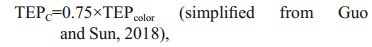
where TEPcolor is the concentration of TEP with the unit of μg Xeq./L.
Linear regression, Pearson correlation, and covariance were performed by Microsoft Excel 2016 software. Dominance index (Eq.3) was used to describe phytoplankton dominant species under this equation:
 (3)
(3)where, N is the total cell abundance of all species, ni is total cell of species i and fi is the count of occurrence of species i in all sample (Guo et al., 2014). Carbon biomass was calculated by following Eqs.4 & 5 (Yang et al., 2016). They were found suitable with current datasets and relatable relationships. They were as follows:
 (4)
(4) (5)
(5)where C represents the amount of carbon (μg). Carbon biomass was computed using 0.011 μg C/trichome as the conversion factor for genus Trichodesmium (Carpenter, 1983).
Canonical correspondence analysis (CCA) were done by Canoco software (version 4.14) among biotic and abiotic parameters of nSCS after performing Detrended Correspondence Analysis (DCA) with respected eigen values. (Ter-Braak and Šmilauer, 2002). Golden Software's Surfer program (https://support.goldensoftware.com/hc/en-us/categories/115000653807-Surfer) was used for integration and visualization of all recorded and examined parameters. Vertical concentrations of different parameters were shown by Ocean Data View (ODV) 4.7.6 software (https://odv.awi.de/en/). T-S diagrams were mentioned to understand the correlations of biotic parameters and TEP with associated water masses.
3 RESULT 3.1 Hydrobiology of SCS transectSeasonal characteristics of nSCS summer was observed during present investigation. Applying horizontal segmentations, high temperature (Fig. 2b) and high salinity (Fig. 2c) were found in the open SCS than on-shelf stations during summer. Vertically, temperature (ranged 14.25–29.95 ℃) was high in surface area (29.34±0.89 ℃). Low salinity was found at the surface of on-shelf stations (Fig. 2a), especially near the estuarine stn. A9 (23.62). High concentration of PO4 were found at the open SCS near the mid transect (Fig. 3a). Average PO4 and SiO4 concentration were 1.3 and 7.02 μmol/L, respectively. Furthermore, average nitrite (Fig. 3b) and SiO4 (Fig. 3d) were comparatively low at Stns. J3 and J4 near MSC (Fig. 1b). Average NO2 and NO3 were 0.21 and 5.33 μmol/L, accordingly (Fig. 3b & c). Vertically, surface of estuarine stations were highly concentrated with nutrients except PO4 (Fig. 4). It was found high at the bottom of the open SCS (Fig. 4d) followed by nitrite (Fig. 4a) and SiO4 (Fig. 4c), especially at Stns. K2 and K4. For better understanding, POC data was extracted by SatCO2 software from satellite data collections. According to the satellite data, POC concentration was found high (100 mg/m3) near estuarine station and low (50 mg/m3) in open nSCS (Supplementary Fig.S1).

|
| Fig.3 Average concentrations of various parameters at all stations in the study area (surface view by software Surfer 12) a. PO4 (μmol/L); b. NO3 (μmol/L); c. NO2 (μmol/L); d. SiO4 (μmol/L); e. phytoplankton (cells/L); f. chl a (μL); g. TEP (μg Xeq./L); h. TEPC (μg C/L). |

|
| Fig.4 Average nutrients concentrations at different depths across SCS |
Phytoplankton assemblages (Fig. 2d) were mainly composed of 3 groups i.e. cyanobacteria (Fig. 2e), diatoms (Fig. 2f), and dinoflagellates (Fig. 2g). Average abundances of phytoplankton were 16 318 cells/L of which approximately 90% was contributed from diatoms (average 14 652 cells/L) and about 10% were cyanobacteria. Average concentration of dinoflagellates was very low at the study area (1.08 cells/L). Dominant phytoplankton species were Trichodesmium thiebautii, Skeletonema costatum (Greville) Cleve, Chaetoceros brevis, Thalassionema nitzschioides (Grunow) Mereschkowsky, Pseudo-nitzschia delicatissima (Cleve) Heiden, Pseudo-nitzschia pungens (Grunow et Cleve) Hasle, Chaetoceros compressus, C. lorenzianus Grunow, and C. pelagicus Cleve. It was observed that average concentration of phytoplankton (Fig. 3e), especially cyanobacteria (average 1 659 cells/L) was high at on-shelf stations (Fig. 2e). Chlorophyll a was also followed similar horizontal patterns of phytoplankton as well. Vertically, it was high at the SCM of Stns. J4 and J5 (average 0.13 μg/L) and in deep water layer of Stns. I1–K4 (Fig. 2h). Horizontally, it was found higher at stations of the shelf area (Fig. 3f).
Through the on-shelf transect, dominant phytoplankton species were Nitzschia sp., S. costatum (Greville) Cleve, T. nitzschioides (Grunow) Mereschkowsky, P. delicatissima (Cleve) Heiden, T. thiebautii, and T. erythraeum Ehrenberg ex Gomont. The open SCS stations possessed T. nitzschioides, Bacteriastrum comosum J. Pavillard, C. messanense Castracane, C. atlanticus var. skeleton Hustedt, C. psedodichaeta Ikari, T. thiebautii, and T. erythraeum as dominant species. Estimations of phytoplankton carbon biomass (Phyto-C) demonstrated higher cyanobacteria (Fig. 5b), especially T. thiebautii through on-shelf segment (Fig. 5d). Phytoplankton, mostly all dominant diatoms were higher at Stn. A9 (Fig. 5a), especially S. costatum (Fig. 5e) and C. brevis (Fig. 5f). Dinoflagellates were less abundant through all stations generally (Fig. 5c). T. nitzschioides (Fig. 5g) and P. pungens (Fig. 5i) were less diverse with high biomass at on-shelf stations. High abundances with low biomass of C. compressus (Fig. 5j), C. lorenzianus (Fig. 5k), and C. pelagicus (Fig. 5l) were found through whole transect.

|
| Fig.5 Carbon biomass of average diatom (a), cyanobacteria (b) and dinoflagellates (c) with average biomass of dominant phytoplankton species, i.e., Trichodesmium thiebautii (d), Skeletonema costatum (e), Chaetoceros brevis (f), Thalassionema nitzschioides (g), Pseudo-nitzschia delicatissima (h), Pseudo-nitzschia pungens (i), Chaetoceros compressus (j), Chaetoceros lorenzianus (k), and Chaetoceros pelagicus (l) |
T-S diagram segmented the on-shelf data into two water masses (Fig. 6a), i.e., high temperature high salinity (HTHS) and low temperature high salinity (LTHS). The open SCS demonstrated two water masses (Fig. 6g), i.e., high temperature low salinity (HTLS) and low temperature high salinity (LTHS). Phytoplankton concentration was higher at LTHS (Fig. 6b) of on-shelf area and at HTLS of the open SCS (Fig. 6h), followed by diatom (Fig. 6c & i) and cyanobacteria as well (Fig. 6e & k). On the other hand, dinoflagellates were distributed less but pretty evenly (Fig. 6d & j) through both zones (on shelf and the open SCS).

|
| Fig.6 T-S plots with depths (a, g) and assemblages of phytoplankton (b, h), diatom (c, i), dinoflagellates (d, j), cyanobacteria (e, k), and TEP concentration (f, l) of on-shelf (a, b, c, d, e, and f) and the open SCS segments (g, h, i, j, k, and l) |
Average TEP concentration (Fig. 2i) was not constant after applying layered segmentation on study transect (58.32±30.56 μg Xeq./L). Horizontally, high TEP was found at the mid transect (Stns. J4 & I1) and at the end of open SCS in average (Fig. 3g). The highest and the lowest recorded TEP was 140.77 and 9.44 μg Xeq./L, respectively. Average vertical concentration of TEP was higher in BSCM (64.99± 36.69 μg Xeq./L) than MLD (62.43±32.15 μg Xeq./L) and SCM (50.67±25.40 μg Xeq./L). Additionally, TEPC showed similar gradients as TEP accordingly (Figs. 2j & 3h). The highest TEPC was 105.57 μg C/L and the lowest was recorded 7.07 μg C/L in SCM (50–100 m) near open SCS (Fig. 1b). T-S distribution of TEP (Fig. 6f & l) followed the distribution patterns of dinoflagellates (Fig. 6d & j) across both zones (on shelf and the open SCS).
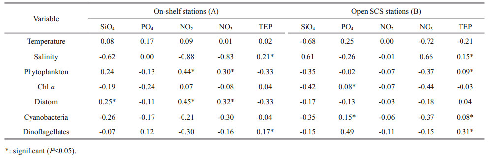
3.4 Correlation of TEP with environmental parametersTEP showed significant positive correlation with cyanobacteria and chl a (P < 0.05) at both horizontal segments through Pearson analysis (Table 1). Positively high coefficients of PO4 with cyanobacteria and dinoflagellates were found at the open SCS as well (Table 1). Following these, CCA also demonstrated close correspondences of TEP with dinoflagellates (Fig. 7a) and cyanobacteria (Fig. 7d), especially with T. thiebautii (Fig. 7b & c). It was also positively correlated with TEP through all water layers. Additionally, CCA also revealed close correspondences of C. pelagicus with concentration of TEP at on-shelf stations (Fig. 7b) and C. compressus at the open SCS (Fig. 7c). CCA showed close relation of depths with chl a through all vertical water layers (Fig. 7d–f). Furthermore, close clustering in group 6 of heatmap (Fig. 8) and linear regression demonstrated significant (R2=0.4) correlations of average TEP with the carbon biomass of cyanobacteria positively (Fig. 9a) and with selected nutrients (SiO4, NO3) negatively (Fig. 9b & c). Supporting these, TEP clustered closely with diatom (Group 1) and cyanobacteria, especially with T. thiebautii (Group 2) after considering their carbon biomass reading as variables during cluster analysis (Fig. 10).

|
| Fig.7 Canonical correspondence analysis (CCA) among biotic and abiotic variables from sampling stations a. average CCA of all variables; b. CCA of variables at on-shelf stations; c. CCA of variables at the open SCS stations; d. CCA of variables in mixed layer depth only; e. CCA of subsurface chlorophyll maximum layers; f. CCA of all variables BSCM. |

|
| Fig.8 Bi-Cluster of sampling stations (Y axis) and various parameters (X axis) of study area with 7 cluster groups Red hue shows positive cluster, yellow are neutral, and green hues are negative clusters from +2.5 to -2.5 in range. |

|
| Fig.9 Linear regression of TEP concentration with cyanobacteria (P=0.03) (a), SiO4 (P=0.03) (b), and nitrite (P=0.03) (c) after 10-based log transformation |

|
| Fig.10 Cluster analysis of TEP with carbon biomass of dominant phytoplankton species |
Bi-Cluster (heat map) analysis expressed close positive (Red hue) and negative (Green hue) relations by considering most of the variables under a correspondence scale from 2.5 to -2.5 (Fig. 8). Diatom dominated phytoplankton was revealed at estuarine station (A9) by close clustering (Group 4). Close cluster of cyanobacteria and TEP were mostly seen at on-shelf stations i.e. J2, J3, and J4 (Group 6). On the other hand, TEP showed average positive correlation with chl a (Y Axis), especially at the open SCS stations i.e. I1 and K3 (Fig. 8; red hue). Additionally, most of positive nutrient clusters (NO3, SiO2, and PO4) were also found here in open SCS (Stns. K2, K4). In summary, bi-cluster analysis indicated that cyanobacteria (in on-shelf stations) and nutrients influenced chl a (at open SCS) were liable of TEP distributions in those horizontal sections accordingly.
A conceptual model was drawn based on results that will be illustrated with references in discussion section (Fig. 11). The text position of each parameters shows highest density of its abundances through the transect. Arrows show uptake of nutrients (green) and influences on TEP (yellow) accordingly. All these relations were built up based on previously described statistical correspondences. Blue dotted circle around monsoon summer currents, indicating a probable mixing impact zone of this throughflow. Slope runoff with nutrients and freshwater (brackish water) from Zhujiang River is indicated by brown dotted arrow. Blue stain in background of Fig. 11 indicates TEP concentrations according to Fig. 2i for better understanding about sources of TEP with high aggregations though the study transects of SCS.

|
| Fig.11 Conceptual model of TEP sourcing at SCS transect |
The largest marginal SCS possessed extreme seasonal variations round the year (Su, 2005; Hu et al., 2014). In summer, weather variations were derived by regional geophysical activities, i.e. flow of MSC and mixing of cyclonic SE through the study area (Hu et al., 2000; Liu et al., 2010; He et al., 2015). The past 32 years' research showed that the intensity of the SCS summer-monsoon (SCSSM) was low while sea surface study temperature was high (Choi et al., 2016). On the other hand, its intensity is higher at the south part of SCS (Tian and Wang, 2010) with the influence of western Pacific weather and ENSO (Mao and Chan, 2005; Ding et al., 2018) followed by Kuroshio (Fig. 1b). All these local phenomena may influence the distributions of TEP and other environmental parameters accordingly. Therefore, understanding local circulations at this transect is important.
During summer, formation of double gyre was seen (Xu et al., 2008) with an eastward MSC, minor eddy (ME) and summer eddy (SE) (Hu et al., 2000; Liu et al., 2010; He et al., 2015) through the study transect (Fig. 1). These geophysical circulations actively played a role in particle distributions (i.e. TEP) and pumping the biological carbon export (Wurl et al., 2009, 2011). All these circulations can act as potential nutrients sources to local biodiversity (Wong et al., 2007). Current study observed low vertical concentration of biotic parameters near the zone (Stns. K4 and SEATS) of cyclonic SE (Fig. 3). It may cause due to the effect of upwelling edge on phytoplankton (Xie, 2003; Yang et al., 2013) and wave mixing in MLD (Huangfu et al., 2018). On the other hand, vertical concentration of TEP, PO4, and chl a were found higher near MSC zone (Stns. J2–J5). Present study predicted that shelf upwelling of nutrient (PO4) may influence chl a (phytoplankton) to produce TEP in this transect (Wong et al., 2007; Gan et al., 2009). Additionally, the concentration of all nutrients (Fig. 3b–d) except PO4 (P; Fig. 3a) and phytoplankton groups (Fig. 2) were higher at the MLD of continental shelf (Fig. 1) near shore (Fig. 2a). It was reported that zonal nutrient enrichments were liable behind these scenario (Xue et al., 2016). In short, nutrients circulations are controlled by geological phenomenon at SCS (Gan et al., 2009) which acted as controlling factors for biotic productions of SCS (Peng et al., 2006).
4.2 TEP correspondence in various environmentsDiatom blooms (Mari, 1999) as well as Cyanobacteria i.e. Anabaena flos-aquae (Surosz et al., 2006), Prochlorococcus marinus (Iuculano et al., 2017), and Synechococcus elongatus (Thornton and Chen, 2017) are potential TEP source (Berman-Frank et al., 2007). Similar to the previous report (Xue et al., 2016), present study found T. thiebautii as dominant cyanobacteria in both sections (on-shelf and the open SCS). This species also showed close relation with concentration of TEP in CCA (Fig. 7b & c). Besides, TEP clustered with cyanobacteria (Fig. 8, Group 6), especially with T. thiebautii accordingly (Fig. 10). These may conclude that T. thiebautii influenced TEP concentration beside diatoms across nSCS (Passow, 2002; Wurl et al., 2011). Significant linear regression of cyanobacteria with TEP (R2=0.42, F=2.86) also support these statements accordingly (Fig. 9a).
Phytoplankton communities were affected by various zonal environmental parameters, especially nutrients during summer (Peng et al., 2006; Ma and Sun, 2014). Upwelling and eddies also had impact on phytoplankton growth (Chen et al., 2006) which may influence TEP production as well (Passow, 2002). Supporting this, bi-cluster analysis (heat map) showed that TEP made a close cluster with phytoplankton (Fig. 8) rather than with nutrients. Additionally, both CCA and Pearson correlation showed significant correspondent between chl a and TEP as well (Table 1). However, it was an opposite statement of some open ocean reports (Wurl et al., 2011; Kodama et al., 2014).
Similarly, Hong et al. (1997) reported the highest range of concentration of TEP in Ross Sea due to high nutrient low productivity (HNLP) under icecaps (Table 2). In BSCM of nSCS (100–200 m), TEP clustered closely with dissolved nutrients (NO3, P, and Si) in CCA (Fig. 7f) which was also consented by Wurl et al. (2011). High sinking rate to TEP may liable behind this scenario after coagulation from extracellular release (Mari et al., 2017). This marked the limitation of current study, which should be addressed in future research.

Geographically, the SCS is influenced by western Pacific currents (Tseng et al., 2016). Reports said that geophysical circulation had potential roles in abundance and variations of phytoplankton as well as particle distributions (Ortega-Retuerta et al., 2009; Liu et al., 2016). Present study found that MLD possessed high TEP (Fig. 2i) and nitrates (Fig. 3c) at on-shelf stations (Fig. 11). Similarly, MLD of Neuse, Jiulong, and Zhujiang River estuaries as well as semiclosed Arabian Sea were also demonstrated moderately high TEP under coastal influences (Prieto et al., 2006; Peng and Huang, 2007; Wetz et al., 2009; Sun et al., 2010). MLD of close seas, i.e. Mediterranean, were also showed high TEP (OrtegaRetuerta et al., 2010; Bar-Zeev et al., 2011) than open ocean (Pacific) due to nutrients limitation on phytoplankton abundances by oligotrophic circulations (Wurl et al., 2011; Kodama et al., 2014). Reports (Table 2) said that the highest TEP concentration was found in Adriatic Sea (Radić et al., 2005). Terrestrial inputs were liable behind this scenario (Kodama et al., 2014; Shu et al., 2018). Similar influential factor from Zhujiang River (Ni et al., 2008; Sun et al., 2010) may cause high concentration of TEP (Fig. 2i) at MLD of on-shelf stations accordingly (Fig. 11).
Furthermore, high cyanobacteria were found in SCM of on-shelf stations (Fig. 2e). It showed close correspondence with TEP in CCA (Fig. 7e). Therefore, cyanobacteria may liable for the high concentration of TEP through this layer (Fig. 11) which was supported by previous report as well (Surosz et al., 2006). High TEP was also found at I1 (Fig. 3g), especially at 200 m (Fig. 2i). This zone is decorated with slope runoff from Zhujiang River (Sun et al., 2010) and shelf upwelling as well (Xie et al., 2003; Yang et al., 2013). Present study also found high NOx (NO2+NO3) concentration at the bottom of on-shelf stations (Fig. 4a & b), which may cause high chl-a concentration in BSCM (Xue et al., 2016). Eventually, this scenario leads to high TEP aggregation across this zone (Passow, 2002; Wurl et al., 2011) in BSCM.
Beside those, current study found high phytoplankton abundances in HTHS and HTLS zone of whole transect (Fig. 6). Additionally, high TEP was found in high diatom (Fig. 6c & i) and high cyanobacteria (Fig. 6e & k) dominated areas as well. They have potential influences on TEP formations in waterbody (Surosz et al., 2006; Thornton et al., 2016). It was reported that temperature showed significant positive correlations with phytoplankton groups during summer in nSCS (Xue et al., 2016). Therefore, temperature may also intrigue TEP sourcing indirectly.
4.4 Assumptions on carbon contributionSCS is acting as CO2 source with carbon exhaustion about 13.86–33.60 Tg C/a (Jiao et al., 2018). POC is a part of that cycle. Studies of POC was mostly focused on phytoplankton cell (Turner, 2002) and zooplankton fecal pellets rather than on TEPC (Turner, 2015). Recent study found that TEPC is a dominant contributor in POC pool (Yamada et al., 2015). It was also suggested that results of TEP should consider in intensive POC study (Guo and Sun, 2018). This study calculated an average 58% contribution of TEPC in POC at the study transect and more than 70% at the open SCS area. It was closely ranged to open Atlantic Ocean (66%) in recent study (Zamanillo et al., 2019). However, it was higher than previous studies (Passow et al., 2001; Mari et al., 2017). High concentrations of phytoplankton and TEP were liable behind this scenario (Passow, 2002). Additionally, high Phyto-C, especially cyanobacteria (Fig. 5b) can also act as a correspondent to POC pool (Bhaskar and Bhosle, 2006; Ortega-Retuerta et al., 2009; de Vicente et al., 2010). Significant positive linearity of TEP with cyanobacteria supported these phenomena (Fig. 9a). Moreover, high POC/TEPC ratio was found in gulf stream (1.5) and slope water (1.4) of western north Atlantic (Jennings et al., 2017), which was similar to the ration at open SCS (1.4) in this study. It signifies intensive influences of TEPC on POC in term of open seawater.
Near nSCS coast, we observed 24.77% TEPC of POC after analyzing satellite data. It was much lower than previous investigation (30%) in the Santa Barbara Channel (Passow et al., 2001) and southern Spain reservoir (Mari et al., 2017). Various particle exporting coastal processes (sediment input, turbidity, mineral flow etc.) can influences these phenomena, which may reduce contribution of TEPC on POC across SCS shore (He et al., 2016). Besides, export of TEP had compatibility with phytoplankton cell sedimentation, which indicates the relationship of them and its importance in POC studies (Guo and Sun, 2018). Therefore, further research should be done on the sinking rate of TEP in SCS and its adjacent sea area after considering regional geophysical activities as well.
5 CONCLUSIONVarious geophysical factors, i.e. SCSSM intensity, local current circulations and adjacent eddies' pumping and regional nutrient upwelling may influence particle distribution pattern (i.e., TEP) and partial carbon abundance (i.e., TEPC) at nSCS. A complex relation of TEP with biological factors and nutrients were also demonstrated by correlation analysis. A number of controlling factors acted separately in different sections of nSCS for TEP concentration. In average, present study found significant positive correlation of TEP with diatom and cyanobacteria i.e. T. thiebautii through various multivariate analysis. It indicates potential influences of them on TEP sourcing. Besides, average TEPC was higher at the deep in the open SCS than on-shelf area. It increases mentionable contribution of TEPC on POC at open water. Further TEP export studies can amplify more about these relations at nSCS.
6 DATA AVAILABILITY STATEMENTAll data generated and/or analyzed during this study are available from the corresponding author on reasonable request.
7 ACKNOWLEDGMENTAuthors express the gratitude to the captain and crews of the R/V Shi Yan 1 for their helps on sampling and on-deck operations, also to Haijiao LIU, Xue BING, and Yi SHU.
Electronic supplementary materialSupplementary material (Supplementary Fig.S1) is available in the online version of this article at https://doi.org/10.1007/s00343-020-0236-x.
Alldredge A L, Passow U, Logan B E. 1993. The abundance and significance of a class of large, transparent organic particles in the ocean. Deep Sea Research Part I: Oceanographic Research Papers, 40(6): 1131-1140.
DOI:10.1016/0967-0637(93)90129-Q |
Bar-Zeev E, Berman T, Rahav E, Dishon G, Herut B, Kress N, Berman-Frank I. 2011. Transparent exopolymer particle(TEP) dynamics in the eastern Mediterranean Sea. Marine Ecology Progress Series, 431: 107-118.
DOI:10.3354/meps09110 |
Bar-Zeev E, Berman-Frank I, Stambler N, Domínguez E V, Zohary T, Capuzzo E, Meeder E, Suggett D J, Iluz D, Dishon G, Berman T. 2009. Transparent exopolymer particles (TEP) link phytoplankton and bacterial production in the Gulf of Aqaba. Aquatic Microbial Ecology, 56(2-3): 217-225.
|
Berman-Frank I, Rosenberg G, Levitan O, Haramaty L, Mari X. 2007. Coupling between autocatalytic cell death and transparent exopolymeric particle production in the marine cyanobacterium Trichodesmium. Environmental Microbiology, 9(6): 1415-1422.
DOI:10.1111/j.1462-2920.2007.01257.x |
Bhaskar P V, Bhosle N B. 2006. Dynamics of transparent exopolymeric particles (TEP) and particle-associated carbohydrates in the Dona Paula bay, west coast of India. Journal of Earth System Science, 115: 403-413.
DOI:10.1007/BF02702869 |
Burd A B, Jackson G A. 2009. Particle aggregation. Annual Review of Marine Science, 1: 65-90.
DOI:10.1146/annurev.marine.010908.163904 |
Carpenter E J. 1983. Physiology and ecology of marine plankton Oscillatoria (Trichodesmium). Marine Biology Letters, 4: 69-85.
|
Chen C C, Kwo S F, Chung S W, Liu K K. 2006. Winter phytoplankton blooms in the shallow mixed layer of the South China Sea enhanced by upwelling. Journal of Marine Systems, 59(1-2): 97-110.
DOI:10.1016/j.jmarsys.2005.09.002 |
Chin W C, Orellana M V, Verdugo P. 1998. Spontaneous assembly of marine dissolved organic matter into polymer gels. Nature, 391(6667): 568-572.
DOI:10.1038/35345 |
Choi J W, Kim B J, Zhang R H, Park K J, Kim J Y, Cha Y, Nam J C. 2016. Possible relation of the western North Pacific monsoon to the tropical cyclone activity over western North Pacific. International Journal of Climatology, 36(9): 3334-3345.
DOI:10.1002/joc.4558 |
Corzo A, Rodríguez-Gálvez S, Lubian L, Sangrá P, Martínez A, Morillo J A. 2005. Spatial distribution of transparent exopolymer particles in the Bransfield Strait, Antarctica. Journal of Plankton Research, 27(7): 635-646.
DOI:10.1093/plankt/fbi038 |
de Vicente I, Ortega-Retuerta E, Mazuecos I P, Pace M L, Cole J J, Reche I. 2010. Variation in transparent exopolymer particles in relation to biological and chemical factors in two contrasting lake districts. Aquatic Sciences, 72(4): 443-453.
DOI:10.1007/s00027-010-0147-6 |
Ding R Q, Li J P, Tseng Y H, Li L J, Sun C, Xie F. 2018. Influences of the North Pacific Victoria Mode on the South China Sea summer monsoon. Atmosphere, 9(6): 229.
DOI:10.3390/atmos9060229 |
Engel A, Passow U. 2001. Carbon and nitrogen content of transparent exopolymer particles (TEP) in relation to their Alcian Blue adsorption. Marine Ecology Progress Series, 219: 1-10.
DOI:10.3354/meps219001 |
Engel A. 2002. Direct relationship between CO2 uptake and transparent exopolymer particles production in natural phytoplankton. Journal of Plankton Research, 24(1): 49-53.
DOI:10.1093/plankt/24.1.49 |
Engel A. 2004. Distribution of transparent exopolymer particles (TEP) in the northeast Atlantic Ocean and their potential significance for aggregation processes. Deep Sea Research Part I: Oceanographic Research Papers, 51(1): 83-92.
DOI:10.1016/j.dsr.2003.09.001 |
Gan J P, Cheung A, Guo X G, Li L. 2009. Intensified upwelling over a widened shelf in the northeastern South China Sea. Journal of Geophysical Research: Oceans, 114(C9): C09019.
|
García C M, Prieto L, Vargas M, Echevarría F, García-Lafuente J, Ruiz J, Rubín J P. 2002. Hydrodynamics and the spatial distribution of plankton and TEP in the Gulf of Cádiz (SW Iberian Peninsula). Journal of Plankton Research, 24(8): 817-833.
DOI:10.1093/plankt/24.8.817 |
Guo S J, Fe ng, Y Y, Wang L, Dai M H, Liu Z L, Bai Y, Sun J. 2014. Seasonal variation in the phytoplankton community of a continental-shelf sea: the East China Sea. Marine Ecology Progress Series, 516: 103-126.
DOI:10.3354/meps10952 |
Guo S J, Sun J. 2018. Sinking rates and export flux of transparent exopolymer particles (TEPs) in an eutrophic coastal sea: a case study in the Changjiang (Yangtze River) estuary. BioRxiv, 357053, https://doi.org/10.1101/357053.
|
He L J, Mukai T, Chu K H, Ma Q, Zhang J. 2015. Biogeographical role of the Kuroshio Current in the amphibious mudskipper Periophthalmus modestus indicated by mitochondrial DNA data. Scientific Reports, 5: 15645.
DOI:10.1038/srep15645 |
He W, Chen M L, Schlautman M A, Hur J. 2016. Dynamic exchanges between DOM and POM pools in coastal and inland aquatic ecosystems: a review. Science of the Total Environment, 551-552: 415-428.
DOI:10.1016/j.scitotenv.2016.02.031 |
Hong Y, Smith W O Jr, White A M. 1997. Studies on transparent exopolymer particles (TEP) produced in the Ross Sea(Antarctica) and by Phaeocystis antarctica(Prymnesiophyceae). Journal of Phycology, 33(3): 368-376.
DOI:10.1111/j.0022-3646.1997.00368.x |
Hu J Y, Kawamura H, Hong H S, Qi Y Q. 2000. A review on the currents in the South China Sea: seasonal circulation, South China Sea Warm Current and Kuroshio intrusion. Journal of Oceanography, 56(6): 607-624.
DOI:10.1023/A:1011117531252 |
Hu Z F, Tan Y H, Song X Y, Zhou L B, Lian X P, Huang L M, He Y H. 2014. Influence of mesoscale eddies on primary production in the South China Sea during spring intermonsoon period. Acta Oceanologica Sinica, 33(3): 118-128.
DOI:10.1007/s13131-014-0431-8 |
Huangfu J L, Chen W, Wang X, Huang R H. 2018. The role of synoptic-scale waves in the onset of the South China Sea summer monsoon. Atmospheric Science Letters, 19(11): e858.
DOI:10.1002/asl.858 |
Iuculano F, Mazuecos I P, Reche I, Agustí S. 2017. Prochlorococcus as a possible source for transparent exopolymer particles (TEP). Frontiers in Microbiology, 8: 709.
DOI:10.3389/fmicb.2017.00709 |
Jennings M K, Passow U, Wozniak A S, Dennis A, Hansell D A. 2017. Distribution of transparent exopolymer particles(TEP) across an organic carbon gradient in the western North Atlantic Ocean. Marine Chemistry, 190: 1-12.
DOI:10.1016/j.marchem.2017.01.002 |
Jiao N Z, Liang Y T, Zhang Y Y, Liu J H, Zhang Y, Zhang R, Zhao M X, Dai M H, Zhai W D, Gao K S, Song J M, Yuan D L, Li C, Lin G H, Huang X P, Yan H Q, Hu L M, Zhang Z H, Wang L, Cao C J, Luo Y W, Luo T W, Wang N N, Dang H Y, Wang D X, Zhang S. 2018. Carbon pools and fluxes in the China Seas and adjacent oceans. Science China Earth Sciences, 61(11): 1535-1563.
DOI:10.1007/s11430-018-9190-x |
Kodama T, Kurogi H, Okazaki M, Jinbo T, Chow S, Tomoda T, Ichikawa T, Watanabe T. 2014. Vertical distribution of transparent exopolymer particle (TEP) concentration in the oligotrophic western tropical North Pacific. Marine Ecology Progress Series, 513: 29-37.
DOI:10.3354/meps10954 |
Liu H J, Xue B, Feng Y Y, Zhang R, Chen M R, Sun J. 2016. Size-fractionated chlorophyll a biomass in the northern South China Sea in summer 2014. Chinese Journal of Oceanology Limnology, 34(4): 672-682.
DOI:10.1007/s00343-016-5017-1 |
Liu S M, Li R H, Zhang G L, Wang D R, Du J Z, Herbeck L S, Zhang J, Ren J L. 2011. The impact of anthropogenic activities on nutrient dynamics in the tropical Wenchanghe and Wenjiaohe Estuary and Lagoon system in East Hainan, China. Marine Chemistry, 125(1-4): 49-68.
DOI:10.1016/j.marchem.2011.02.003 |
Liu Z F, Li X J, Colin C, Ge H M. 2010. A high-resolution clay mineralogical record in the northern South China Sea since the Last Glacial Maximum, and its time series provenance analysis. Chinese Science Bulletin, 55(35): 4058-4068.
DOI:10.1007/s11434-010-4149-5 |
Ma L L, Chen M, Guo L D, Lin F, Tong J L. 2012. Distribution and source of transparent exopolymer particles in the northern Bering sea. Acta Oceanologica Sinica, 34(5): 81-90.
(in Chinese with English abstract) |
Ma W, Sun J. 2014. Characteristics of phytoplankton community in the northern South China Sea in summer and winter. Acta Ecologica Sinica, 34(3): 621-632.
(in Chinese with English abstract) |
Malpezzi M A, Sanford L P, Crump B C. 2013. Abundance and distribution of transparent exopolymer particles in the estuarine turbidity maximum of Chesapeake Bay. Marine Ecology Progress Series, 486: 23-35.
DOI:10.3354/meps10362 |
Mao J Y, Chan J C L. 2005. Intraseasonal variability of the South China Sea summer monsoon. Journal of Climate, 18(13): 2388-2402.
DOI:10.1175/JCLI3395.1 |
Mari X, Passow U, Migon C, Burd A B, Legendre L. 2017. Transparent exopolymer particles: effects on carbon cycling in the ocean. Progress in Oceanography, 151: 13-37.
DOI:10.1016/j.pocean.2016.11.002 |
Mari X. 1999. Carbon content and C: N ratio of transparent exopolymeric particles (TEP) produced by bubbling exudates of diatoms. Marine Ecology Progress Series, 183: 59-71.
DOI:10.3354/meps183059 |
Miller M J, Chikaraishi Y, Ogawa N O, Yamada Y, Tsukamoto K, Ohkouchi N. 2013. A low trophic position of Japanese eel larvae indicates feeding on marine snow. Biology Letters, 9: 20120826.
DOI:10.1098/rsbl.2012.0826 |
Ni H G, Lu F H, Luo X L, Tian H Y, Zeng E Y. 2008. Riverine inputs of total organic carbon and suspended particulate matter from the Pearl River Delta to the coastal ocean off South China. Marine Pollution Bulletin, 56(6): 1150-1157.
DOI:10.1016/j.marpolbul.2008.02.030 |
Ortega-Retuerta E, Duarte C M, Reche I. 2010. Significance of bacterial activity for the distribution and dynamics of transparent exopolymer particles in the Mediterranean Sea. Microbial Ecology, 59(4): 808-818.
DOI:10.1007/s00248-010-9640-7 |
Ortega-Retuerta E, Reche I, Pulida-Villena E, Agustí S, Duarte C M. 2009. Uncoupled distributions of transparent exopolymer particles (TEP) and dissolved carbohydrates in the Southern Ocean. Marine Chemistry, 115(1-2): 59-65.
DOI:10.1016/j.marchem.2009.06.004 |
Passow U, Alldredge A L, Logan B E. 1994. The role of particulate carbohydrate exudates in the flocculation of diatom blooms. Deep Sea Research Part I: Oceanographic Research Papers, 41(2): 335-357.
DOI:10.1016/0967-0637(94)90007-8 |
Passow U, Alldredge A L. 1994. Abiotic formation of transparent exopolymer particles (TEP) from polysaccharides excreted by phytoplankton. Abstr. Pap.Am. Chem. Soc., 207: 1-78.
|
Passow U, Alldredge A L. 1995. A dye-binding assay for the spectrophotometric measurement of transparent exopolymer particles (TEP). Limnology and Oceanography, 40(7): 1326-1335.
DOI:10.4319/lo.1995.40.7.1326 |
Passow U, Shipe R F, Murray A, Pak D K, Brzezinski M A, Alldredge A L. 2001. The origin of transparent exopolymer particles (TEP) and their role in the sedimentation of particulate matter. Continental Shelf Research, 21(4): 327-346.
DOI:10.1016/S0278-4343(00)00101-1 |
Passow U. 2000. Formation of transparent exopolymer particles, TEP, from dissolved precursor material. Marine Ecology Progress Series, 192: 1-11.
DOI:10.3354/meps192001 |
Passow U. 2002. Transparent exopolymer particles (TEP) in aquatic environments. Progress in Oceanography, 55(3-4): 287-333.
DOI:10.1016/S0079-6611(02)00138-6 |
Peng A G, Huang Y P. 2007. Study on TEP and its relationships with uranium, thorium, polonium isotopes in Jiulong Estuary. Journal of Xiamen University (Natural Science), 46(S1): 38-42.
(in Chinese with English abstract) |
Peng X, Ning X R, Sun J, Le F F. 2006. Responses of phytoplankton growth on nutrient enrichments in the northern South China Sea. Acta Ecologica Sinica, 26(12): 3959-3968.
(in Chinese with English abstract) |
Prieto L, Navarro G, Cózar A, Echevarría F, García C M. 2006. Distribution of TEP in the euphotic and upper mesopelagic zones of the southern Iberian coasts. Deep Sea Research Part II: Topical Studies in Oceanography, 53(11-13): 1314-1328.
DOI:10.1016/j.dsr2.2006.03.009 |
Radić T, Kraus R, Fuks D, Radić J, Pečar O. 2005. Transparent exopolymeric particles' distribution in the northern Adriatic and their relation to microphytoplankton biomass and composition. Science of the Total Environment, 353(1-3): 151-161.
DOI:10.1016/j.scitotenv.2005.09.013 |
Ramaiah N, Yoshikawa T, Furuya K. 2001. Temporal variations in transparent exopolymer particles (TEP) associated with a diatom spring bloom in a subarctic Ria in Japan. Marine Ecology Progress Series, 212: 79-88.
DOI:10.3354/meps212079 |
Shu Y, Zhang G C, Sun J. 2018. The distribution and origin of transparent exopolymer particles at the PN section in the East China Sea. Haiyang Xuebao, 40(8): 110-119.
(in Chinese with English abstract) |
Sibuet J C, Yeh Y C, Lee C S. 2016. Geodynamics of the South China Sea. Tectonophysics, 692: 98-119.
DOI:10.1016/j.tecto.2016.02.022 |
Su J L. 2005. Overview of the South China Sea circulation and its dynamics. Acta Oceanologica Sinica, 27(6): 1-8.
(in Chinese with English abstract) |
Sun C C, Wang Y S, Li Q P, Yue W Z, Wang Y T, Sun F L, Peng Y L. 2012. Distribution characteristics of transparent exopolymer particles in the Pearl River estuary, China. Journal of Geophysical Research: Biogeosciences, 117(G4): G00N17.
DOI:10.1029/2012JG001951 |
Sun C C, Wang Y S, Wu M L, Li N, Lin L, Somg H, Wang Y T, Deng C, Peng Y L, Sun F L, Li C L. 2010. Distribution of transparent exopolymer particles in the Pearl River estuary in summer. Journal of Topical Oceanography, 29(5): 81-87.
(in Chinese with English abstract) |
Sun J, Liu D Y, Qian S B. 2002. A quantative research and analysis method for marine phytoplankton: an introduction to Utermöhl method and its modification. Journal of Oceanography of Huanghai & Bohai Seas, 20(2): 105-112.
(in Chinese with English abstract) |
Surosz W, Palińska K A, Rutkowska A. 2006. Production of transparent exopolymer particles (TEP) in the nitrogen fixing cyanobacterium Anabaena flos-aquae Ol-K10. Oceanologia, 48(3): 385-394.
|
Ter-Braak C J F, Šmilauer P. 2002. CANOCO Reference Manual and CanoDraw for Windows User's Guide: Software for Canonical Community Ordination (Version 4. 5). Microcomputer Power, Wageningen.
|
Thornton D C O, Brooks S D, Chen J. 2016. Protein and carbohydrate exopolymer particles in the sea surface microlayer (SML). Frontiers of Marine Science, 3: 135.
|
Thornton D C O, Chen J. 2017. Exopolymer production as a function of cell permeability and death in a diatom(Thalassiosira weissflogii) and a cyanobacterium(Synechococcus elongatus). Journal of Phycology, 53(2): 245-260.
DOI:10.1111/jpy.12470 |
Tian Y, Wang Q. 2010. Definition of the South China Sea summer monsoon onset. Chinese Journal of Oceanology and Limnology, 28(6): 1281-1289.
DOI:10.1007/s00343-010-9950-0 |
Tseng Y H, Lin H Y, Chen H C, Thompson K, Bentsen M, Böning C W, Bozec A, Cassou C, Chassignet E, Chow C H, Danabasoglu G, Danilov S, Farneti R, Fogli P G, Fujii Y, Griffies S M, Ilicak M, Jung T, Masina S, Navarra A, Patara L, Samuels B L, Scheinert M, Sidorenko D, Sui C H, Tsujino H, Valcke S, Voldoire A, Wang Q, Yeager S G. 2016. North and equatorial Pacific Ocean circulation in the CORE-II hindcast simulations. Ocean Modelling, 104: 143-170.
DOI:10.1016/j.ocemod.2016.06.003 |
Turner J T. 2002. Zooplankton fecal pellets, marine snow and sinking phytoplankton blooms. Aquatic Microbial Ecology, 27: 57-102.
DOI:10.3354/ame027057 |
Turner J T. 2015. Zooplankton fecal pellets, marine snow, phytodetritus and the ocean's biological pump. Progress in Oceanography, 130: 205-248.
DOI:10.1016/j.pocean.2014.08.005 |
Vicente Villardón J L. 2015. MULTBIPLOT: A package for Multivariate Analysis using Biplots. Departamento de Estadística. Universidad de Salamanca.
|
Welschmeyer N A. 1994. Fluorometric analysis of chlorophyll a in the presence of chlorophyll b and pheopigments. Limnology and Oceanography, 39(8): 1985-1992.
DOI:10.4319/lo.1994.39.8.1985 |
Wetz M S, Robbins M C, Paerl H W. 2009. Transparent exopolymer particles (TEP) in a river-dominated estuary: spatial-temporal distributions and an assessment of controls upon TEP formation. Estuaries and Coasts, 32(3): 447-455.
DOI:10.1007/s12237-009-9143-2 |
Wong G T F, Ku T L, Mulholland M, Tseng C M, Wang D P. 2007. The Southeast Asian time-series study (SEATS) and the biogeochemistry of the South China Sea-An overview. Deep Sea Research Part II: Topical Studies in Oceanography, 54(14-15): 1434-1447.
DOI:10.1016/j.dsr2.2007.05.012 |
Wurl O, Holmes M. 2008. The gelatinous nature of the seasurface microlayer. Marine Chemistry, 110(1-2): 89-97.
DOI:10.1016/j.marchem.2008.02.009 |
Wurl O, Miller L, Röttgers R, Vagle S. 2009. The distribution and fate of surface-active substances in the sea-surface microlayer and water column. Marine Chemistry, 115(1-2): 1-9.
DOI:10.1016/j.marchem.2009.04.007 |
Wurl O, Miller L, Vagle S. 2011. Production and fate of transparent exopolymer particles in the ocean. Journal of Geophysical Research: Oceans, 116(C7): C00H13.
|
Xie S P, Xie Q, Wang D X, Liu W T. 2003. Summer upwelling in the South China Sea and its role in regional climate variations. Journal of Geophysical Research: Oceans, 108(C8): 3261.
DOI:10.1029/2003JC001867 |
Xu H, Xie S P, Wang Y, Zhuang W, Wang D. 2008. Orographic effects on South China Sea summer climate. Meteorology and Atmospheric Physics, 100(1-4): 275-289.
DOI:10.1007/s00703-008-0309-4 |
Xue B, Sun J, Li T T. 2016. Phytoplankton community structure of northern South China Sea in summer of 2014. Haiyang Xuebao, 38(4): 54-65.
(in Chinese with English abstract) |
Yamada Y, Fukuda H, Uchimiya M, Motegi C, Nishino S, Kikuchi T, Nagata T. 2015. Localized accumulation and a shelf-basin gradient of particles in the Chukchi Sea and Canada Basin, western Arctic. Journal of Geophysical Research: Oceans, 120(7): 4638-4653.
DOI:10.1002/2015JC010794 |
Yang H Y, Wu L X, Liu H L, Yu Y Q. 2013. Eddy energy sources and sinks in the South China Sea. Journal of Geophysical Research: Oceans, 118(9): 4716-4726.
DOI:10.1002/jgrc.20343 |
Yang Y, Sun X X, Zhu M L, Luo X, Zheng S. 2016. Estimating the carbon biomass of marine net phytoplankton from abundance based on samples from China seas. Marine and Freshwater Research, 68(1): 106-115.
DOI:10.1071/MF15298 |
Zamanillo M, Ortega-Retuerta E, Nunes S, Rodríguez-Ros P, Dall'Osto M, Estrada M, Montserrat Sala M, Simó R. 2019. Main drivers of transparent exopolymer particle distribution across the surface Atlantic Ocean. Biogeosciences, 16: 733-749.
DOI:10.5194/bg-16-733-2019 |