 2021, Vol. 39
Institute of Oceanology, Chinese Academy of Sciences
Article Information
- ZHANG Yongshun, FENG Miao, ZHANG Weimin, WANG Huizan, WANG Pinqiang
- A Gaussian process regression-based sea surface temperature interpolation algorithm
- Journal of Oceanology and Limnology, 39(4): 1211-1221
- http://dx.doi.org/10.1007/s00343-020-0062-1
Article History
- Received Jan. 21, 2020
- accepted in principle Apr. 21, 2020
- accepted for publication Oct. 20, 2020


2 Key Laboratory of Software Engineering for Complex Systems, National University of Defense Technology, Changsha 410073, China
Ocean reanalysis datasets can improve the accuracy of ocean studies by assimilating observational data, so they are widely used in studies of ocean thermal and dynamic processes and their spatiotemporal variability (Du and Qu, 2010; Kumar and Hu, 2012; Balmaseda et al., 2013). They can also provide initial conditions and side boundary conditions for model simulation and prediction. Research regarding the development of high-resolution ocean reanalysis datasets and associated applications is therefore very important. However, increasing the resolution of numerical models to improve ocean reanalysis datasets involves using huge quantities of computational resources, especially for global datasets. Low-resolution ocean reanalysis datasets are usually interpolated into higher-resolution regional ocean models using nearest neighbor interpolation, linear interpolation or bicubic interpolation (Nardelli et al., 2016). This has the advantage of a lower calculation cost and can be completed relatively quickly. Other common interpolation methods for data assimilation, such as optimal interpolation and the successive corrections method are also often used to interpolate ocean reanalysis datasets, but these methods require background field information (Wang et al., 2008, 2012). However, although traditional interpolation methods can improve the resolution of ocean reanalysis datasets, they cannot introduce multiscale physical feature information. This is because they do not take into account spatio-temporal changes and non-linear processes. They only use some calculation of adjacent values to interpolate. As a result, the products obtained through interpolation often contain errors (Li and Heap, 2008), especially with regard to coastal waters and the areas around islands (Sokolov and Rintoul, 1999).
In recent years, machine learning methods have been increasingly applied to the interpolation of geographic data. Li et al. (2011) used 23 methods, including random forest and support vector machines, to interpolate mud content samples from the southwestern edge of Australia and compared the different results. The machine learning results were found to be the most accurate. Jia and Ma (2017) applied machine learning methods to the interpolation of seismic data, which can significantly reduce costs in engineering applications. In the field of meteorology, Antonić et al. (2001) used neural networks to interpolate meteorological data. Research has shown that neural networks can accurately simulate complex non-linear functions (Bryan and Adams, 2002), making them suitable for the processing of certain kinds of complex non-linear relationships in data. Appelhans et al. (2015) used multiple machine learning methods to interpolate monthly average temperatures and, in a quantitative evaluation, found the results to be better than the Kriging method. Based on a 10-fold cross-validation testing design, regression trees generally performed better than linear and non-linear regression models.
Out of all the different marine elements, temperature, especially sea surface temperature (SST), has the greatest impact on air-sea interactions (Thompson et al., 2017). In order to reduce the obvious errors of traditional interpolation methods near the offshore area and islands, this paper uses machine learning methods to interpolate SST. There are numerous different machine learning methods. The kernel method can transform linear learning into non-linear learning by introducing a kernel function. This can map linearly inseparable problems in an original sample space to a higher-dimensional feature space where the linearly inseparable problem will be solved (Hofmann et al., 2008). Common machine learning methods for classification or regression that apply kernel functions include support vector machines (SVM), support vector regression (SVR), and gaussian process regression (GPR). In the field of meteorology, kernel methods have also performed well. Wang and Zhang (2005) used weighted least squares support vector machines (WLS-SVMs) to estimate wind speed and found this could accurately track wind speed trends and produce highly accurate estimations. Wang and Chaib-draa (2017) proposed a novel online Bayesian filtering framework for large-scale GPR and applied it to global surface temperature analysis. The results showed that this approach was an efficient and accurate expert system for global surface temperature analysis. Paniagua-Tineo et al. (2011) used SVR to accurately predict the maximum temperature over a period of 24 hours by introducing predictors such as temperature, precipitation, relative humidity, and barometric pressure. Based on statistical tests, the SVR performed better than a Multi-layer perceptron and an Extreme Learning Machine in this prediction problem.
GPR has a strictly theoretical basis for its approach to statistical learning and is adaptable to a range of complex problems, including high dimensionality, small sample size, and nonlinearity. It is also highly generalizable. In comparison to neural networks and support vector approaches, this method has the advantages of easy implementation, adaptive acquisition of hyperparameters, and the probabilistic significance of its outputs (He et al., 2013). It is therefore widely used in the field of image super-resolution (He and Siu, 2011). Improving the spatial resolution of SST through interpolation can actually be compared to image super-resolution. Both obtain higher resolution data from low resolution data. The Gaussian process defines a joint Gaussian distribution for any finite number of samples, which can be used to simulate a random sample distribution of sea surface temperatures.
Various factors can affect the SST (Katsaros et al., 2005), such as the sea surface wind stress, sea surface heat flux, and ocean current velocity. These physical factors have different influence radii and intensities. A single kernel function cannot capture this multi-scale information. A combined kernel function therefore needs to be constructed to extract their different influence radii and intensities. Huang et al. (2014) used SVM models to predict short-term wind speeds and introduced different climate variables as input features to produce ideal prediction results. Grover et al. (2015) used wind direction, spatial distance, pressure, and temperature to infer long-term spatial dependencies through GPR.
Taking all of the above into account, this paper presents the design of an SST interpolation algorithm based on GPR. By constructing a combined kernel function, latitude and longitude, sea surface wind stress, sea surface heat flux, and ocean current velocity are used as input features to establish the regression relationship between these non-linear features and SST, which can effectively reduce the interpolation error near the offshore area and islands.
The remaining sections of the paper are organized as follows: Section 2 introduces the basic principles of GPR, commonly-used kernel functions, multi-scale kernel functions for processing meteorological ocean processes and SST interpolation algorithms based on GPR. Section 3 presents the results of some SST interpolation experiments. The last section gives our overall conclusions.
2 GAUSSIAN PROCESS REGRESSION AND KERNEL FUNCTION 2.1 Gaussian process regressionA Gaussian process can be applied to a set of any finite random variables that obey a joint Gaussian distribution (Rasmussen and Williams, 2006). It can be fully represented by its mean function and covariance function, i.e.:
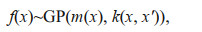
where, GP is an abbreviation for Gaussian process, x and x' are arbitrary random variables, and
For the purposes of simplification, the mean function is typically taken to be 0 (Rasmussen and Williams, 2006).
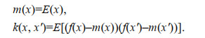
Let us suppose there is a training set, D={(xi, yi)| i=1, 2, …, n}=(X, y), where, x∈Rd is a d-dimensional input vector, and X={x1, x2, …, xn} is a d×n-dimensional input matrix. yi∈R is the corresponding output scalar and y is the output vector. R is a real number field, and Rd is a d-dimensional real number space.
Assuming the training set is noisy, the following model can be used:

If ε~N (0, σn2), we can get the prior distribution of y as follows:
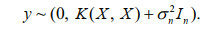
Assuming that y* is the predicted value corresponding to the test point, x*, the joint Gaussian distribution of y and y* can be obtained as follows:

If there are n training points and n* test points, then K(X, x*) represents the n×n* order covariance matrix used to measure the correlation between x and x*. The same is true for K(X, X), K(x*, X), and k(x*, x*). In is an n-dimensional identity matrix, x is the input vector, and N is the distribution.
GPR is a non-parametric algorithm based on Bayesian framework, the Bayesian posterior distribution of y* is:

The mean and variance of the predicted values of corresponding to are:
GPR obtains the entire distribution at the point to be predicted. The mean is then usually chosen as the best regression value.
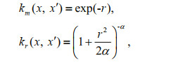
2.2 Kernel functionThe key feature of Gaussian process regression is that the covariance matrix, K, of the joint Gaussian distribution has to be a symmetric semi-definite matrix. In the kernel method, the kernel functions are all symmetric and semi-definite, so, theoretically the kernel functions used in machine learning can be used as covariance matrices. The squared exponential (SE) covariance function is the most commonly used kernel function. It can be expressed as follows:
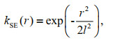
where, l is the length scale, r=x-x', x and x' are the input vectors in the test set and training set, respectively.
The SE covariance function is infinitely differentiable, so, a Gaussian process with this covariance function has mean square derivatives of all orders, making it very smooth and only able to handle single features. This means it is not suitable for modeling complex physical processes (Rasmussen and Williams, 2006).
The rational quadratic (RQ) kernel function differs from the SE covariance function in its ability to handle features with different length scales. It can deliver very fine simulations of various abnormal sea surface temperatures along coasts and near islands. The function can be expressed as follows:
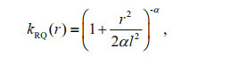
when the hyperparameters l and α are greater than 0, it can be regarded as an infinite scale mixture of the SE covariance function with different length scale features (Rasmussen and Williams, 2006). Thus, it amounts to the sum of multiple kernel functions.
Unlike the smooth characteristics of the SE covariance function, the Matérn class kernel function's characteristics are rough. Its general expression is as follows:
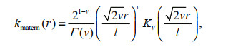
where, l is a length scale hyperparameter; Kv is a modified Bessel function; and Γ is a gamma function. v=p+1/2 (p is a non-negative integer, such as 1, 2, 3, etc). The smaller the value of v, the better the function can handle complex nonlinear relationships. This makes it more suitable for handling meteorological and oceanic processes. Commonly, v=1/2, 3/2, or 5/2.
If v=1/2, the kernel function can be simplified as follows:

It has been proven that the sum, product, and scale of existing kernel functions are still kernel functions (Rasmussen and Williams, 2006). Multi-scale information can be extracted by combining kernel functions, with the appropriate kernel functions being selected and combined according to a combination rule to extract the characteristic information for different physical processes in a targeted fashion. The length-scale hyperparameter l relates to the influence radius of each feature.
2.3 GPR-based interpolation algorithmSST is the result of a combination of thermal, dynamic oceanic processes and air-sea interactions. Due to the complexity and randomness of its influencing factors, the latitude and longitude distribution of SST is uneven. As a result of the influence of the sea surface wind and sea surface heat flux, SST may also be subject to abnormal local phenomena in some areas. Furthermore, it can also be affected by coastal runoff in offshore areas and around islands. At the same time, SST is not entirely chaotic with time. Generally speaking, changes in SST adhere to a significant annual cycle and are seasonally affected (Du et al., 2003).
As similarly spatially located samples have similar distributions, the geographic location (longitude, latitude) can be used as an initial input feature. In view of the physical causes and influencing factors of SST, zonal sea surface wind stress, meridional sea surface wind stress, sea surface heat flux, zonal current velocity, and meridional current velocity can be selected as additional input characteristics.
The Matérn class kernel function is especially well-suited to extraction of the rough feature distribution of SST. The rougher the function, the more detailed the changes that can be extracted. As noted above, the RQ kernel function can be regarded as the sum of numerous SE covariance functions with different length scale features. This function can simultaneously fit a wide range of uniform temperature distributions across the ocean surface and abnormal local temperature changes, including in coastal areas and around islands.
In view of the various factors that can influence SST, a combined kernel function, ks, was constructed to describe the distribution characteristics of SST:
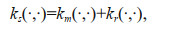
km(·, ·), here, represents a Matérn class kernel function when v=1/2. kr(·, ·) represents an RQ kernel function. Matérn class kernel functions can describe complex non-linear features that affect SST, while the RQ kernel function can describe the distribution characteristics of SST from different shores to distant seas at different scales.
Specifically,
where 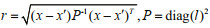
The hyperparameters α and l in the kernel function are both unknown and can be set to 0 until derived from a marginal likelihood logarithm.
The training and prediction process of the interpolation algorithm is shown in Fig. 1.

|
| Fig.1 Algorithm process |
To assess the validity of the proposed approach, we used the Global Ocean Reanalysis Dataset SODA (Simple Ocean Date Assimilation) developed by the University of Maryland and Texas A & M University. The spatial resolution of this product is 0.5°×0.5°; the latitudinal and longitudinal range is 0.25°E-180°- 0.25°W, 74.75°S-89.75°N; and the layers are unequally spaced in a vertical direction, with there being a total of 50 layers. In this paper, the temperature to a depth of 5 m was selected as the SST.
The experiment used monthly data from 2014 to 2015. The study area was 0°-66°N, 100°E-180°. The training set had a resolution of 1°×1° and was sampled from the original data set for the 12 months in 2014. The remaining data was used as the validation set. This selection was chosen to train and obtain hyperparameters from the data of a single month and to explore the effect of monthly and seasonal changes in sea surface temperature on the interpolation effect. Out of these 12 sets of training and validation experiments, the best set of hyperparameters was selected. The data from the South China Sea in May 2015 was then selected as a test set. The experimental process is shown in Fig. 2.

|
| Fig.2 Experimental process |
It should also be noted that, because the focus was the sea surface temperature, invalid values in the land area had to be eliminated. The input variables were the longitude, latitude, zonal sea surface wind stress, meridional sea surface wind stress, sea surface heat flux, zonal current velocity at 5 m, and meridional current velocity at 5 m. The control experiments were bilinear interpolation, bicubic interpolation, nearest neighbor interpolation, Support Vector Regression and Principal Component Regression (hereinafter referred to as Bilinear, Cubic, Nearest, SVR and PCR).
The root mean square error (RMSE) was used to evaluate the accuracy of the interpolation, which can be defined as follows:
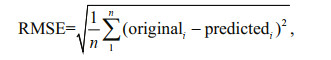
in which, originali is the i-th SST in the original data; predictedi is the i-th predicted value; and n is the number of interpolation points. The RMSE represents the average deviation between the predicted and original values.
As noted above, the SST interpolation results can also easily be described in image form. The structural similarity index (SSIM) is a common indicator for measuring the similarity of two images, so the SSIM can also be used to evaluate the interpolation results. Assuming the two input images are x and y, the SSIM can be defined as:
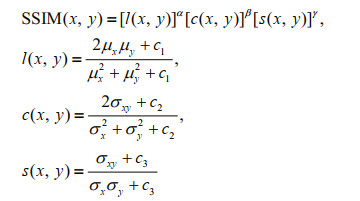
where l(x, y) is the brightness comparison; c(x, y) is the contrast comparison; and s(x, y) is the structural comparison. μx and μy represent the average of x and y; σx and σy represent the standard deviation; and σxy represents the covariance of x and y. c1, c2, and c3 are constants to avoid system errors caused by there being a denominator of 0. Generally, we set α=β=γ=1, c1= 6.502 5, c2=58.522 5, and c3=c2/2 (Wang et al., 2004).
The SSIM range is 0 to 1. The more similar the two images, the greater its value. When the two images are exactly the same, the SSIM value is equal to 1.
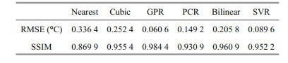
3.1 Results of the single test setThrough the experiments on the validation set, based on the results of the RMSE and SSIM evaluations, it was established that the parameters generated from the training set for September 2014 provided the optimal model, the parameters generated by machine learning include hyperparameters in the mean function, covariance function, and likelihood function. This model was therefore used to predict the test set. Excluding the land area, the test set had 1 397 effective interpolation points. The test area was the South China Sea, as specified above, which will hereinafter be referred to as "Region 1".
It can be immediately seen in Fig. 3 that the interpolation effect using GPR was better than the Bilinear, Cubic, Nearest, and PCR interpolation methods in most areas, especially at the land-sea boundaries. As a kernel machine learning method, the SVR interpolation method had similar advantages as GPR, but it was still slightly worse than the interpolation effect of GPR. The comparative RMSE results in Table 1 show that the RMSE obtained by the GPR interpolation was 62.4% lower than Nearest interpolation, 43.7% lower than Cubic interpolation, and 38.9% lower than Bilinear interpolation.

|
|
Fig.3
Difference between the original SST and the result of a different interpolation
a. the Nearest interpolation; b. the Cubic interpolation; c. the GPR interpolation; d. the PCR interpolation; e. the Bilinear interpolation; f. the SVR interpolation.
The green area is almost 0, indicating that the interpolation result is very close to the original value. |

|
It is noted also that, if the result of the interpolation is exactly the same as the true value, you can draw a graph where all the differences are 0 (i.e., green). If this figure is used as a reference, the SSIM values between the difference map and the reference map generated by the above six methods can be calculated. The difference between the results obtained by the six interpolation methods and the original image can then be measured, as is also shown in Table 1. It was found that the value of the GPR interpolation was still the closest to 1. This shows that, even if the super-resolution accuracy is measured from an image perspective, the GPR interpolation is still better than the other types of interpolation.
3.2 The temporal and spatial generalizability of the interpolation algorithmThe generalizability of a model learned through machine learning refers to the extent to which it can be applied to a new sample. For a spatiotemporally continuous geographic data interpolation algorithm, such as SST, its generalizability needs to be considered in temporal and spatial terms.
As the hyperparameters of the model were generated by training on a single month of data, it is necessary to examine the algorithm's temporal generalizability. It can be seen from Fig. 4 that the results for the Nearest interpolation method were the worst across all 12 months. The GPR interpolation method produced significantly better interpolation results than the other five from March to October, with the interpolation results in September and October being the best. This may be because the hyperparameters of the best model selected in the validation set were for September 2014 and SST has a regular interannual change. The interpolation effect of GPR for each month was consistently better than the other five methods, indicating that the algorithm's temporal generalizability is more reliable than other methods.

|
| Fig.4 The SSTs interpolated by different methods for 2015 in Region 1 |
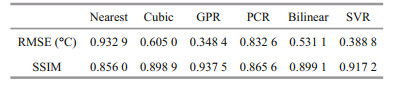
The above experiments were all performed in Region 1. We will now examine the algorithm's spatial generalizability. The test time was unified to May 2015 and two other regions were selected to compare the interpolation results. The selected areas were 0°–30°N, 125°E–150°E and 30°N–65°N, 115°E–150°E (hereinafter referred to as Region 2 and Region 3). Region 2 was just ocean. Region 3 was the sea around both land and an island.
Combining the results shown in Fig. 5 and Table 2, it can be seen that, for the ocean far from land, the GPR interpolation effect is very good, with the RMSE being nearly 70.6% lower than the Bilinear interpolation, 76.0% lower than Cubic interpolation and 81.9% lower than Nearest interpolation. It can also be seen in Fig. 5 that the GPR method was significantly better than the traditional method in the northwestern part of Region 2. This is because this area is located in the south of the island, and the interpolation of GPR method near the island can perform better. Similarly, machine learning methods including SVR and PCR interpolation method also had better interpolation effects in this area than traditional methods.

|
|
Fig.5
The difference between the original SST and those of different interpolations for 2015 in Region 2
a. the Nearest interpolation; b. the Cubic interpolation; c. the GPR interpolation; d. the PCR interpolation; e. the Bilinear interpolation; f. the SVR interpolation.
There were 2 444 valid interpolation points in Region 2. |
|
Combining the results in Fig. 6 and Table 3, it can be seen that, for the ocean near the island, the GPR interpolation effect is still good, with the RMSE being nearly 34.4% lower than the Bilinear interpolation, 42.4% lower than Cubic interpolation and 62.7% lower than Nearest interpolation. However, it can be seen that, in addition to the two kernel machine learning methods, other interpolation methods are less effective near the island.

|
|
Fig.6
The difference between the original SST and those of different interpolations for 2015 in Region 3
a. the Nearest interpolation; b. the Cubic interpolation; c. the GPR interpolation; d. the PCR interpolation; e. the Bilinear interpolation; f. the SVR interpolation.
There were 1 496 valid interpolation points in Region 3. |
|
In summary, the following conclusions can be drawn:
1. The SST interpolation results for the ocean near land and islands is not as good as it is for areas far from land.
2. Overall, GPR interpolation performs better than traditional interpolation (Bilinear, Cubic, and Nearest). The GPR interpolation results are very good, whether the ocean is far from land and islands or at their boundaries.
3. The temporal and spatial generalizability of the GPR interpolation algorithm is reliable.
3.3 The effect of seasonal changes on the algorithmAs the best set of hyperparameters and the corresponding kernel functions selected by the validation set were generated by the training set for September 2014, the temporal generalizability of the interpolation algorithm was found to be best for the test sets for September and October 2015. As the SST is subject to significant change over a 12 month period, we decided to explore the effect of using kernel functions generated by training in similar months.
The experimental setup was as follows. The GPR algorithms generated in February, May, August, and November 2014 were selected to test the data from January to March, April to June, July to September, and October to December 2015. The selected test area was still the South China Sea. The test results were compared with the original interpolation algorithm, the Bilinear interpolation and the Cubic interpolation results.
As can be seen in Fig. 7, the GPRn interpolation performed worse than the original GPR interpolation from March to October, with the interpolation results for the other four months being slightly better. It is therefore worth considering using GPR for interpolation from March to October and GPRn for the remaining four months. Overall, both interpolation effects outperformed the Bilinear interpolation and the Cubic interpolation. However, the results of these tests suggest that the effect of seasonal changes on the GPR interpolation algorithm were not obvious.

|
| Fig.7 Using the original GPR interpolation methods and the GPR interpolation method for generating kernel functions in similar months to interpolate the SST for 2015 in Region 1 GPRn: GPR interpolation results using the kernel function generated in the nearest month. The Cubic interpolation results were used for background reference. |
It can be seen from Fig. 8 that the Bilinear interpolation method, the Cubic interpolation method, and the Nearest interpolation method consume almost the same amount of time. When there were 1 397 effective interpolation points, this was about 20-21 s, with the GPR interpolation method, PCR interpolation method, and SVR interpolation method taking about 22-23 s. Thus, the GPR interpolation method has an additional time cost of about 2 s (10%). In terms of the improved interpolation accuracy, this cost is completely acceptable.

|
| Fig.8 Comparison of the time consumption for the six different interpolation methods for the 12 months of 2015 in Region 1 The software used in the interpolation experiment was Matlab R2016a. As the algorithm runs differently each time, the average time over five runs was taken. |
Improving the spatial resolution of ocean reanalysis datasets is very important for the study of meso-scale and small-scale ocean processes and sea-air interactions. It can also provide initial conditions and side boundary conditions for high-resolution regional models. To reduce the errors introduced by traditional interpolation methods that only use local neighborhood sample points for interpolation, this paper has sought to introduce physical factors such as sea surface wind stress, sea surface heat flux, ocean current velocity, and SST into the design of an interpolation algorithm based on GPR. Here, the GPR interpolation method has focused on the SST in SODA reanalysis products. The results show that this method can significantly reduce the interpolation error. Compared with the nearest neighbor interpolation, bicubic interpolation, and bilinear interpolation methods, it had an RMSE that was 62.4%, 43.7%, and 38.9% lower, respectively. The improvement in the interpolation accuracy was especially obvious for coastal waters and the areas around islands. The algorithm showed good temporal and spatial generalizability. The hyperparameters obtained from the training set data for September 2014 were the best. This set of parameters was able to generate the best interpolation results for other months as well. The model obtained in the training area can also be applied to other regions in the Western Pacific. The South China Sea is affected by monsoons and the circulation is subject to seasonal changes. We therefore also tested the effect of seasonal changes on the algorithm. The results showed that the effect of seasonal changes on the algorithm is not significant.
The study reported here has several shortcomings. There are a number of other factors that affect SST, not all of which we have introduced into the kernel functions. Only the SST in ocean reanalysis datasets was considered. In the future, the interpolation model needs to be extended and interpolation algorithms for sea surface salinity and sea surface height will need to be developed to improve the spatial resolution of ocean reanalysis datasets in a more comprehensive way. The interpolation algorithm can also be extended below the sea surface to interpolate ocean elements such as temperature and salinity at various depths, thus enabling high-resolution display of three-dimensional oceanic processes. This would facilitate a more accurate description of dynamic ocean processes and the development of more accurate models to ascertain initial field and boundary conditions.
5 DATA AVAILABILITY STATEMENTThe datasets generated during and/or analyzed during the current study are available from the corresponding author on reasonable request.
6 ACKNOWLEDGMENTWe are grateful to the University of Maryland and Texas A & M University for developing, maintaining and making available (https://www.atmos.umd.edu/~ocean/) the SODA datasets that were used in this study.
Antonić O, Križan J, Marki A, Bukovec D. 2001. Spatiotemporal interpolation of climatic variables over large region of complex terrain using neural networks. Ecological Modelling, 138(1-3): 255-263.
DOI:10.1016/S0304-3800(00)00406-3 |
Appelhans T, Mwangomo E, Hardy D R, Hemp A, Nauss T. 2015. Evaluating machine learning approaches for the interpolation of monthly air temperature at Mt. Kilimanjaro, Tanzania. Spatial Statistics, 14: 91-113.
DOI:10.1016/j.spasta.2015.05.008 |
Balmaseda M A, Trenberth K E, Källén E. 2013. Distinctive climate signals in reanalysis of global ocean heat content. Geophysical Research Letters, 40(9): 1 754-1 759.
DOI:10.1002/grl.50382 |
Bryan B A, Adams J M. 2002. Three-Dimensional Neurointerpolation of Annual Mean Precipitation and Temperature Surfaces for China. Geographical Analysis, 34(2): 93-111.
DOI:10.1111/j.1538-4632.2002.tb01078.x |
Du Y, Qu T D. 2010. Three inflow pathways of the Indonesian throughflow as seen from the simple ocean data assimilation. Dynamics of Atmospheres and Oceans, 50(2): 233-256.
DOI:10.1016/j.dynatmoce.2010.04.001 |
Du Y, Wang D, Xie Q, Church J. 2003. Harmonic analysis of sea surface temperature and wind stress in the vicinity of the maritime continent. Acta Meteorologica Sinica, 17(S1): 226-237.
|
Grover A, Kapoor A, Horvitz E. 2015. A deep hybrid model for weather forecasting. In: Proceedings of the 21th ACM SIGKDD International Conference on Knowledge Discovery and Data Mining. ACM, Sydney. p. 379-386, https://doi.org/10.1145/2783258.2783275.
|
He H, Siu W C. 2011. Single image super-resolution using Gaussian process regression. In: Proceedings of CVPR 2011. IEEE, Providence. p. 449-456, https://doi.org/10.1109/CVPR.2011.5995713.
|
He Z K, Liu G B, Zhao X J, Yang J. 2013. Temperature model for FOG zero-bias using Gaussian process regression. In: Du Z Y ed. Intelligence Computation and Evolutionary Computation. Springer, Berlin. p. 37-45, https://doi.org/10.1007/978-3-642-31656-2_6.
|
Hofmann T, Schölkopf B, Smola A J. 2008. Kernel methods in machine learning. The Annals of Statistics, 36(3): 1 171-1 220.
DOI:10.1214/009053607000000677 |
Huang R L, Yu Z, Deng Y C, Zeng X L. 2014. Short-term wind speed forecasting based on SVM under different feature vectors. Acta Energiae Solaris Sinica, 35(5): 866-871.
(in Chinese with English abstract) DOI:10.3969/j.issn.0254-0096.2014.05.022 |
Jia Y N, Ma J W. 2017. What can machine learning do for seismic data processing? An interpolation application. Geophysics, 82(3): V163-V177.
DOI:10.1190/geo2016-0300.1 |
Katsaros K B, Soloviev A V, Weisberg R H, Luther M E. 2005. Reduced horizontal sea surface temperature gradients under conditions of clear skies and weak winds. BoundaryLayer Meteorology, 116(2): 175-185.
DOI:10.1007/s10546-004-2421-4 |
Kumar A, Hu Z Z. 2012. Uncertainty in the ocean-atmosphere feedbacks associated with ENSO in the reanalysis products. Climate Dynamics, 39(3-4): 575-588.
DOI:10.1007/s00382-011-1104-3 |
Li J, Heap A D, Potter A, Daniell J J. 2011. Application of machine learning methods to spatial interpolation of environmental variables. Environmental Modelling & Software, 26(12): 1 647-1 659.
DOI:10.1016/j.envsoft.2011.07.004 |
Li J, Heap A D. 2008. A Review of Spatial Interpolation Methods for Environmental Scientists. Geoscience Australia, Canberra. 137p.
|
Nardelli B B, Droghei R, Santoleri R. 2016. Multi-dimensional interpolation of SMOS sea surface salinity with surface temperature and in situ salinity data. Remote Sensing of Environment, 180: 392-402.
DOI:10.1016/j.rse.2015.12.052 |
Paniagua-Tineo A, Salcedo-Sanz S, Casanova-Mateo C, OrtizGarcía E G, Cony M A, Hernández-Martín E. 2011. Prediction of daily maximum temperature using a support vector regression algorithm. Renewable Energy, 36(11): 3 054-3 060.
DOI:10.1016/j.renene.2011.03.030 |
Rasmussen C E, Williams C K I. 2006. Gaussian Processes for Machine Learning. MIT Press, Cambridge. 248p.
|
Sokolov S, Rintoul S R. 1999. Some Remarks on interpolation of Nonstationary oceanographic fields. Journal of Atmospheric and Oceanic Technology, 16(10): 1 434-1 449.
DOI:10.1175/1520-0426(1999)016<1434:SROION>2.0.CO;2 |
Thompson B, Tkalich P, Malanotte-Rizzoli P. 2017. Regime shift of the South China Sea SST in the late 1990s. Climate Dynamics, 48(5-6): 1 873-1 882.
DOI:10.1007/s00382-016-3178-4 |
Wang H Z, Wang G H, Chen D K, Zhang R. 2012. Reconstruction of three-dimensional pacific temperature with Argo and satellite observations. Atmosphere-Ocean, 50(S1): 116-128.
DOI:10.1080/07055900.2012.742421 |
Wang H Z, Zhang R, Liu W, Wang G H, Jin B G. 2008. Improved interpolation method based on singular spectrum analysis iteration and its application to missing data recovery. Applied Mathematics and Mechanics, 29(10): 1 351-1 361.
DOI:10.1007/s10483-008-1010-x |
Wang Q J, Zhang X F. 2005. Effective wind speed estimation for variable speed wind turbines based on WLS-SVM. Journal of System Simulation, 17(7): 1 590-1 593.
(in Chinese with English abstract) DOI:10.3969/j.issn.1004-731X.2005.07.017 |
Wang Y L, Chaib-draa B. 2017. An online Bayesian filtering framework for Gaussian process regression: application to global surface temperature analysis. Expert Systems with Applications, 67: 285-295.
DOI:10.1016/j.eswa.2016.09.018 |
Wang Z, Bovik A C, Sheikh H R, Simoncelli E P. 2004. Image quality assessment: from error visibility to structural similarity. IEEE Transactions on Image Processing, 13(4): 600-612.
DOI:10.1109/TIP.2003.819861 |