 2023, Vol. 41
Institute of Oceanology, Chinese Academy of Sciences
Article Information
- WU Pengfei, WU Lin, BAO Lifeng, WANG Long, WANG Bo, TANG Danling
- A marine gravimeter based on electromagnetic damping and its tests in the South China Sea
- Journal of Oceanology and Limnology, 41(2): 792-803
- http://dx.doi.org/10.1007/s00343-022-2110-5
Article History
- Received Mar. 23, 2022
- accepted in principle May 4, 2022
- accepted for publication Jul. 21, 2022


2 University of the Chinese Academy of Sciences, Beijing 100049, China;
3 Guangdong Remote Sensing Center for Marine Ecology and Environment (GDRS), Southern Marine Science and Engineering Guangdong Laboratory (Guangzhou), Guangzhou 511458, China;
4 School of Geography and Information Engineering, China University of Geosciences, Wuhan 430074, China
Relative gravity meters such as the JMGrav marine gravimeter directly measure the force of the Earth's gravity field beneath the sensor. Changes in gravity correlate directly to changes in density, which makes gravity sensors valuable tools in detecting, modelling, and interpreting subsurface anomalies due to faults, mineral deposits, and water, gas, and oil reservoirs as well as the geoid (Torge, 1989). Gravity sensors are extremely sensitive accelerometers that measure in static differences in the order of 1 part in 100 million of the Earth's gravitational field (Riccardi et al., 2002). In a dynamic ocean environment, however, the vertical accelerations caused by waves and currents are much larger than those caused by gravity. Many experiences have shown that the excursions of the measuring system of a marine gravimeter located in a research vessel are so large that the measurements very often cannot be evaluated at all. It was therefore suggested that a design be made in such a manner that measurements suitable for evaluation would be possible with vertical accelerations of up to 100 Gal (1 Gal=10-2 m/s2) in magnitude and with periods of up to 15 s (Geyer and Ashwell, 1992).
Consequently, it became necessary to increase the damping of the marine gravimeter considerably. The damping system of a typical Lacoste and Romberg (Ander et al., 1999; Carbone and Rymer, 1999; Abbasi et al., 2007) type marine gravimeter utilizes a complex air damper consisting of interleaving concentric cylinders to restrain high frequency vertical accelerations. To damp the pendulum motion in the Chekan-AM gravimeter (Krasnov et al., 2014a; Forsberg et al., 2015), the housing of the elastic system consisting of two torsion systems made of high purity quartz glass is filled with organic silicon fluid to provide its damping (Krasnov et al., 2014b). Both air and fluid damping systems are limited by an inability of the instrument housing to perfectly deal with thermal compensation and pressure isolation and has significant gravity amplitude reduction and time delay. In recent years, Dynamic Gravity Systems (DGS) (Tinto et al., 2019; Zhang et al., 2020) and Gravimetric Technologies (GT) (Bolotin and Yurist, 2011; Abramov and Koneshov, 2015; Golovan et al., 2018) have developed electromagnetic damping technology. This damping substantially attenuates vertical accelerations and is insensitive to temperature and pressure changes. In the Lacoste and DGS beam-type gravimeters, however, apparent gravity can be distorted over each cycle of ship motion when horizontal and vertical components of acceleration have equal periods and are out of phase. A cross-coupling of the acceleration components then occurs, reaching maximum effects for 90° phase differences. In the GT gravimeter, a non-linear correction is required due to the asymmetric mass-spring system.
A new electromagnetic damping gravity sensor was developed for the marine gravimeter JMGrav developed and produced by the Innovation Academy for Precision Measurement Science and Technology, Chinese Academy of Sciences. The essential developments of the gravity sensor are presented in this paper. The force distribution and damping effects of the system were studied, and the dynamic characteristics of the system under different motion conditions were simulated. Special attention was given to the time lag and amplitude reduction of the instrument indication when the vessel passes over a gravity anomaly. Then, the gravity measurements with a JMGrav marine gravimeter onboard the R/V Dongfanghong 3 during a survey in the South China Sea were obtained. Finally, the measurement data were evaluated, and the gravity survey results are presented.
2 DESIGN AND METHOD 2.1 Sensor designThe gravity sensor is the core part of the JMGrav marine gravimeter and is used to accurately measure the acceleration of gravity. The constant gravity acceleration g0 is compensated by a metal zerolength spring made of constant modulus alloy, whereas gravity changes are detected by the electromagnetic system.
The mass-spring system (Fig. 1), which is based on an axially symmetric sensor, consists of a cylinder-shaped mass guided by 6 threads in frictionless manner. The motion of the mass is limited to one degree of freedom in vertical direction. Therefore, horizontal accelerations do not affect the motion and the sensor is free from any CrossCoupling errors.

|
| Fig.1 Schematic diagram of the gravity sensor |
The frictionless guidance of the mass is achieved by means of the tensioned threads that lead the mass system vertically. From the outer frame, 6 horizontal threads in two planes perpendicular to the mass axis are tangentially fixed on the cylinder-shaped mass in a 120° configuration. These threads are tensioned by a pair of springs in a 180° configuration. An optimum tensioning is very important in respect of system sensibility and sensitivity to external perturbing acceleration. The symmetric burdened threads under static conditions are loaded by additional forces under horizontal acceleration. The dimensions of the cross-section are selected to ensure linear measuring conditions up to high acceleration values.
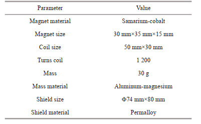
The damping system consists of a movable coil situated at the lower part of the mass in the field of two pairs of strong permanent magnets. The coil is wound along the mass axis, the winding of the coil is rectangular, and its normal line is perpendicular to the mass axis. The strong permanent magnets are made of samarium cobalt, which has very good temperature stability, a high coercivity and a high magnetic energy product, and a low inflection point in the demagnetization curve, which produces a highly stable and uniform magnetic field.
Figure 2 details the functional components of the electromagnetic damping. A pair of magnets is mounted horizontally reversed to the axis of the mass, with the air gap between the two magnets encompassing the upper horizontal part of the coil winding. The magnetic induction is parallel to the coil normal. The other pair of magnets is mounted in the lower part of the coil winding, in the same vertical plane as the two magnets above. The magnetic induction of the upper and lower pairs of magnets is of equal magnitude and in exactly opposite directions and is approximately uniform. The main geometric dimensions and physical parameters of the damper are shown in Table 1.

|
| Fig.2 Schematic diagram of the electromagnetic damping |
The coil fixed to mass, in the permanent magnetic field, is displaced in the vertical direction when subjected to changes in gravity or vertical accelerations. The magnetic damping is produced by a change in the magnetic flux of the coil due to mass motion. A high level of damping is achieved without the use of liquids. This damping is augmented with circuit damping via sophisticated servo techniques.
The servo electronics include excitation oscillator, precision differential capacitive displacement transducer, servo amplifier, and feedback servo compensation circuits. The capacitive transducer is mounted at the top of the mass, where it detects extremely small displacements of the mass with respect to the outer casing of the sensor. The servo electronics produce a proportional electrical current through the coil in response to the transducer signal. The resulting electromagnetic force equal and opposite to the applied acceleration exactly balances the inertial reactive forces. The mass displacement is greatly reduced to less than 3 μm, whereby superimposed disturbing accelerations in the vertical direction are damped by the electrical damping. Meanwhile, the servo electronics produce an integral electrical current which drives the mass displacement to zero, and also suppresses vertical accelerations. The current passing through the coil is thus an exact measure of gravity variations.
Most of the delicate parts of the sensor are inside a special containment, a Dewar-vessel, to protect them against sudden temperature changes. A grid of heating wires is attached to the Dewar-vessel, which together with control-electronics keeps the internal temperature at a constant level of approximately 50 ℃. The temperature shift is less than 0.01 ℃. To reduce magnetic disturbances coming from external fields an extra magnetic shielding is installed. In addition, a pressure-sealed case is provided to prevent changes in air-pressure from entering the sensor.
2.2 Performance analysis 2.2.1 Analysis of the mass-spring systemThe sensor operates as a zero-method system. The mass is always fed back to an absolute geometric null. All six horizontal threads and a pair of tension springs are perpendicular to the main spring and the force on the mass in the vertical direction is zero, at which point the sensitivity of the mass-spring system is equal to that of the main spring. As the open loop gain of the servo amplifier cannot be infinite, the spring mass assembly deviates from zero when subjected to vertical accelerations. The deflection breaks the mutual perpendicularity, the main spring and all threads and tension springs act together in the vertical direction on the mass, at which point the sensitivity of the mass-spring system is equal to an equivalent sensitivity:
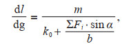 (1)
(1)where, m is the mass, k0 is the stiffness of the main spring, Fi is the tension of the threads and restraint springs, b is the deflection from geometric null, and α is the angle between the threads and the horizontal.
Also, the deflection of mass with respect to the absolute geometric null results in the CrossCoupling errors:
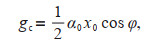 (2)
(2)where, α0 is the amplitude of angular motion between the threads and the horizontal, x0 is the amplitude of the horizontal acceleration x, φ is phase difference between α and x.
The angular motion α is very small due to the mass displacement is greatly reduced to less than 3 μm by damping, so the Cross-Coupling errors can be ignored.
In fact, the mass rotates slightly as it moves. This rotation will also cause the main spring to distort, so that the torque caused by mass rotation is applied directly to the main spring, causing instability in the sensor. The mass-spring system is therefore suspended from the outer casing of the sensor by a very thin twisted wire.
2.2.2 Analysis of the electromagnetic field characteristicsThe finite element software ANSYS electromagnetic field simulation and analysis module was used to analyze the internal magnetic field of the damping system. The method of simulating the damping characteristics of the system based on the ANSYS 3D electromagnetic field transient analysis method provides a basis for optimizing the performance of the damper. When velocity effects are considered for the three-dimensional simulation model of the electromagnetic field, harmonic analysis and transient analysis can be carried out. Harmonic analysis can only be applied to a constant magnetic field. Therefore, in this study, a three-dimensional transient analysis was carried out in which the constant magnetic field generated by the permanent magnet was equated to a time-varying load. Figures 3 & 4 show the magnetic induction and magnetic flux of the electromagnetic system, respectively.

|
| Fig.3 Magnetic induction of the electromagnetic system |

|
| Fig.4 Magnetic flux of the electromagnetic system |
The vertical motion of the coil in the permanent magnetic field generates an induced electromotive force and an induced current. Meanwhile, the servo electronics produce a proportional current through the coil in response to the differential capacitor signal. Both currents generate electromagnetic forces in the magnetic field. The simulation results of the damping performance of the electromagnetic system are given in Table 2.
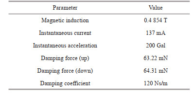
In Table 2, the damping force F:
 (3)
(3)induced the electromotive force E:
 (4)
(4)and induced the current Ie:
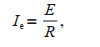 (5)
(5)where, n is coil turns, B is the magnetic induction, l is the length of the coil in the permanent magnetic field, v is the movement velocity of the coil in vertical direction, R is coil resistance. The current Ic in response to the differential capacitor depends on the displacement of the mass, here the displacement is taken as 3 μm.
2.2.3 Evaluation of sensitivity and accuracy in staticThe sensor has been first tested in static conditions. The measurement uncertainty has been estimated to 0.05 mGal (1 mGal=10-5 m/s2). The estimation of the uncertainties has been confirmed by the comparison with a CG6 gravimeter. The measurement sensitivity of the sensor in static is equal to 0.1 mGal Hz-. Figure 5 shows long-period observations made by the sensor on the ground. Although affected by ground vibration and other factors, a relatively obvious tidal curve can still be observed.

|
| Fig.5 Comparison of the statically observed curve with the tide model |
Owing to the heavy damping the apparent gravity change ∆g* corresponding to a mass displacement x is not equal to the true gravity change ∆g. This discrepancy will now be examined. To do this, the equation of motion is needed:
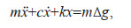 (6)
(6)where m, k, and c are the mass of the detection electrode and the mass, the equivalent stiffness of the elastic system, and the damping of the electromagnetic system, respectively. Two gravity variations will now be examined: gravity anomalies represented respectively, by a step change and a sinusoidal change.
The height difference between floors is used to generate gravity anomalies to simulate step gravity changes. The gravity sensor is placed in an elevator and then quickly taken from the first floor to the seventh floor, resulting in a sudden gravity change. The outputs of the gravimeter are observed to test the responses of the instrument to the gravity anomalies caused by the elevation differences. The observed steady-state responses of the sensor are shown in Table 3.
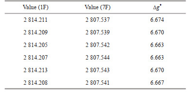
|
Table 3 shows that the mean value of the measured gravity anomalies is 6.665 mGal, and the measured height difference ∆h between the first floor and the seventh floor is approximately 21.5 m. When the elevation of the measuring point is less than 1 000 m, the free air correction usually uses the simplified correction formula ∆g=0.308 6 ∆h, and the theoretical value of 6.635 mGal is basically consistent with the observed value. The heavier damping results in an increase in the running-in period. For a sudden change in gravity ∆g, an exponential response of the measuring system is obtained.
The response curve is shown in Fig. 5; the time constant, i.e., the time constant in which the measured value changes by the fraction (l–l/e) of its ultimate change ∆g, now amounts to approximately 1– 2 min. Step change from g to g+∆g (Fig. 6). The following equation is derived.
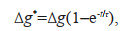 (7)
(7)

|
| Fig.6 Response curve of a sudden gravity change ∆g |
which means that the response is exponential with the time constant τ.
This shows that the time constant τ, which is proportional to the damping force, can readily be determined from Eq.7. Rapid changes in floor height, e.g., in 2–3 s, by a definite amount; the instrument will reach a new value tracing a nearly exponential curve. By fitting the response curve to the most suitable exponential function, the time constant τ can readily and accurately be found.
In the Fig. 6, the measuring system approaches a new value along an exponential curve (blue line). The time constant τ is a measure of the initial slope of the curve (dotted line). The sinusoidal gravity change, taking into consideration Eq.6, may be expressed as follows:
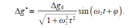 (8)
(8)With τ=100 s, it follows from Eq.8 that for periods T from 1 s to approximately 30 s. The dependence of the damping attenuation ratio upon T is approximately linear:
 (9)
(9)Compared with the effect of damping at shorter periods, the longer periods are of greater importance. The question now arising is by what amount a gravity anomaly impressed upon the gravimeter is reduced owing to heavy damping. To simplify mathematics, a gradually rising and falling gravity anomaly (salt dome) will be represented as a single period of a sine wave, from the trough through the crest to the trough.
When a research vessel travelling at a velocity of 18 km/h (approximately 10 knots) passes over a salt dome-type gravity anomaly extending over 3 km, the gravity change acting upon the marine gravimeter corresponds to a sine wave with a period of 600 s. With this value and the time constant τ=100 s, the attenuation ratio ∆g*/∆g=0.95 is illustrated in Fig. 7.

|
| Fig.7 Response curves to a sinusoidal gravity change |
Thus, the recording will not show the true value of the anomaly but only an amplitude reduced to 95%. For different ship velocities and extensions of the anomaly, different periods will be obtained. Consequently, local anomalies of small extent should always be traversed with as small a velocity as possible unless provision is made to apply corrections to the recorded values.
In addition to the amplitude reduction, damping will also result in an indication lag ∆t. For a sinusoidal gravity change, the indication lag is given by:
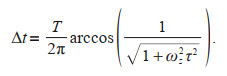 (10)
(10)The response to a sinusoidal gravity change can also been tested on a motion simulator, the up and down motions of which are practically sinusoidal. The so-called sine motion simulator used provides simple harmonic motions with amplitudes up to 250 cm and periods of 5–1 000 s. For a period of 10 s this would mean that gravity variations (vertical accelerations) would reach peaks of 100 Gal. The gravimeter was subjected to simulated sinusoidal gravity changes having periods of 5–1 000 s with a break of 1 000 s between each test. The values of the damping attenuation ratio and the indication lag are given in Table 4.
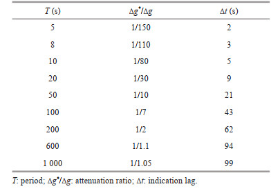
The dependence of the attenuation ratio and indication lag upon the impressed period T, according to the data indicated by the recorder, are illustrated in Fig. 8. We notice that for τ=100 s, the true value of the measured gravity does not significantly change during periods of more than 1 000 s. If the periods are greater than 1 000 s, the indication lag practically equals the time constant τ, but it decreases rapidly for shorter periods.

|
| Fig.8 Amplitude reduction factor for sinusoidal gravity changes (a) and indication lag for sinusoidal gravity changes (b) |
It was found from Fig. 8 that the amplitude reduction of vertical accelerations with periods of 3–15 s is 30–45 dB (the value is calculated by formula 20log ∆g*/∆g), while the effect on gravity with periods greater than 600 s is less than 0.5 dB. In actual operation, the research vessel generally travels at a speed of 10 knots or less, and most of the periods of gravity anomalies will exceed 12 000 s. The amplitude reduction of the gravity signal can be ignored.
Another important question in the marine gravimeter records is whether the measured value is independent of the vertical acceleration produced by the state of the sea, in other words, whether the marine gravimeter will indicate, despite the continually impressed alternating vertical accelerations the same average value as it would when these vertical accelerations were absent, i.e., with the instrument completely at rest although located on the same site and at the same elevation.
The requirements that a marine gravimeter must meet can only be satisfied if the indications are, to very close limits, linearly dependent upon the impressed vertical accelerations within a very large range. The tests of the marine gravimeter on the simulator show that a practically ideal linearization is attained. For periods between 5 and 10 s and accelerations up to 100 Gal, the discrepancies between the static and dynamic responses do not exceed 1 mGal.
Figure 9 shows an example of linearization. The tracing runs upwards, and indicates, first, the responses to vertical acceleration amplitudes of 100 Gal at periods of 5 s; next, the static responses are shown, and then the responses to vertical acceleration at periods of 8 and 10 s. Since the state of the sea will, in general, change only slightly within a few hours, the small residual discrepancies may cause errors, but probably of not more than 1 mGal.

|
| Fig.9 Example of a gravimeter recording responses to periodic up and down motions imparted to the sensor over large sine lifts |
A JMGrav Marine gravimeter was installed on board the Ocean University of China R/V Dongfanghong 3 (Fig. 10) in September 2020 in Sanya, Hainan Province. A marine gravity survey was conducted in northern South China Sea (Table 5). The instrument comes in a rugged housing, containing gravity sensor, gyro-stabilized platform, control electronics, power supply, and shock absorbing mounts. Gravity measurements on board a ship must be carried out on a stabilized platform to eliminate the effects of roll and pitch. A gyro-stabilized platform has been designed to meet the requirements for the dynamic accuracy of the JMGrav gravimeter (Wu et al., 2017). It consists of a gimbal mounting comprising two frames. One frame is placed inside the other by means of roller bearings. Each frame is made for one axis of rotation, i.e., pitch and roll respectively. The sensor itself is placed exactly in the middle of the two gimbal axes. A special gyro together with a biaxial horizontal accelerometer provides correction signals to be fed into two motors. The motors quickly rotate the frames back to their horizontal position.

|
| Fig.10 JMGrav marine gravimeter used in R/V Dongfanghong 3 |
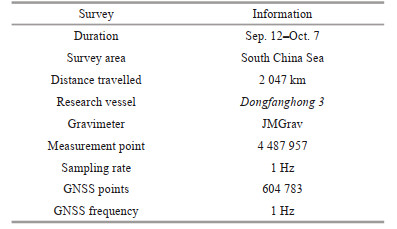
The instrument was located near the intersection of the longitudinal and transverse axes of the ship, with the pitch and roll axes of the platform aligned parallel to the longitudinal and lateral vehicle axes, respectively. A high-precision inertial navigation system (INS) and a Global Navigation Satellite System (GNSS) receiver were installed adjacent to the gravimeter to obtain the position, navigation, acceleration, and attitude information. All data were collected and stored in the acquisition system of the gravimeter to ensure time synchronization of the measured data.
The voyage departed on September 12 and proceeded to the survey area by an almost direct route. The track of Dongfanghong 3 during the survey is shown in Fig. 11, and the effective survey line exceeds 2 000 km. Sea conditions varied from calm to slight-to-moderate swells during the tests. Occasionally, sea conditions were harsh, with an acceleration of more than 200 Gal. However, this also provided a rare opportunity to test the instrument's adaptability and accuracy in harsh sea conditions and to verify the anti-interference performance of the damping system over a wide range of vertical acceleration disturbance periods. Throughout the entire time of the offshore survey, the instrument was in working order, and its performance was tested over many days of continuous operation.

|
| Fig.11 Track of Dongfanghong 3 during the survey Map review No. GS2022(4314). |
Data from more than 2 000 km were collected during the survey. The data used in this study were obtained on three legs that took the research vessel through a large variety of sea conditions. The important question to be examined first relates to the performance of the damping system if it is not subjected to sinusoidal cycles but rather to irregular alternating vertical accelerations, which in most cases will be the case at sea.
An INS record presented in Fig. 12a shows that the amplitude of vertical accelerations imparted to the gravimeter exceeded 100 Gal with a wide band energy distribution from 1 to 100 s. Figure 12b illustrates the behavior of the gravimeter when almost jerky vertical accelerations were imparted to it. The record shows that the values of the responses were usually less than 1 Gal and response time was less than 3 min, which indicates that the vertical acceleration had been approximately attenuated 40 dB by damping. This test unambiguously demonstrated the high order of performance attainable with the damping system of the JMGrav gravimeter even in the quite irregular states of the seas and swells.

|
| Fig.12 Vertical accelerations (a) and gravimeter raw data (b) |
First, we measured the gravity along a profile crossing the continental slope, the Xisha Trough, the Zhongsha Trough, and the Central Basin where there is an important gravity signal. High accuracy ocean gravity field models were used as references to assess the external coincidence accuracy of the JMGrav gravimeter. The Sandwell and Smith series (S & S) (Sandwell et al., 2014; Lequentrec-Lalancette et al., 2016) from the Scripps Institution of Oceanography, University of California San Diego (SIO), and DTU series (Andersen and Knudsen, 2019; Zhang et al., 2021) from the DTU are typical representative references. Both models are in a state of continuous updating, with the latest releases having an accuracy better than 2 mGal and a spatial resolution of 1′×1′ (Watts et al., 2020; Li et al., 2021). We have, therefore, a very good knowledge of the gravity anomaly along the profile. The measurements on this profile are shown in Fig. 13. The profile is compared to the one obtained by satellite altimetry (Fig. 13a). The difference between the JMGrav measurements and the satellite model S & S V30.1 has a standard deviation of 5.4 mGal and a mean value of -0.17 mGal. In fact, the length of the profile is over 1 200 km. Off level errors derived from the inability of the platform, in which the sensor is mounted, occur when the ship is unable to maintain straight along the survey line. The difference between the two profiles has a standard deviation of 2.9 mGal and a mean value of 0.2 mGal where the ship traveled in a strictly straight line.

|
| Fig.13 Gravity measurements along the profile a. free air gravity anomaly measured by the JMGrav gravimeter and free gravity anomaly from satellite measurements (Sandwell v30.1); b. difference between the JMGrav gravimeter data and the reference data of Sandwell; c. depth along the profile. https://www.gebco.net. |
It is seen from Fig. 13a that the free air anomalies often vary rapidly along the profile. From Fig. 13c it is seen that these variations are very closely related to the changes in bathymetry. The correlation coefficient between the JMGrav gravimeter data and topographic relief was 0.84. The close correlation between water depth and free-air gravity anomaly shown in Fig. 13 is by itself good reason for believing that the gravimeter data are valid.
Then, we measured the gravity along a grid on the Xiannan abyssal sea knoll at the northern Central Basin in the South China Sea. The grid is laid out as shown in Fig. 14, with 6 east-west lines and 2 north-south lines, resulting in 12 crossing points. The gravity differences at the crossing points are shown in Fig. 14a. Such differences in the middle section of the survey lines are relatively small but became appreciable when sustained horizontal accelerations occur as the ship alters course to acquire a new line. Normally, one plans the turn to provide a straight approach to the survey line of 6– 10 min to allow the platform of JMGrav gravimeter to settle. This characteristic tends to be a drawback when surveying in heavy traffic, or where other obstacles demand frequent course changes.

|
| Fig.14 Gravity anomaly model of Xiannan abyssal sea knoll at the northern Central Basin a. the grid layout with the gravity differences at the crossing points; b. model obtained from the JMGrav gravimeter measurements. The blue line in (a) are the profiles on which the gravity was measured. |
The measurement error of this survey has been estimated to 1.3 mGal from the differences at the crossing points (the error is calculated by taking the standard deviation of the differences at the crossing points divided by 
We have designed and developed a new gravity sensor based on electromagnetic damping technology and applied it in a JMGgrav marine gravimeter. A high level of damping is achieved without the use of liquids. This damping is augmented with circuit damping via sophisticated servo techniques. Therefore, on the one hand, it is insensitive to short-period vertical accelerations, and on the other hand, it faithfully reproduces long-period gravity variations. Tests on the dynamic characteristics of the damping system using a motion simulator show that the performance of this damping system has a clear regularity with respect to the period of vertical acceleration in the frequency band from 1 to 1 000 s. The amplitude reduction of the vertical accelerations with periods of 3–15 s is 30–45 dB, with a time lag of 2–5 s, while the effect on gravity with periods greater than 600 s is less than 0.5 dB, with a time lag of less than 100 s.
In September 2020, R /V Dongfanghong 3 conducted a gravity survey with a JMGrav gravimeter in the South China Sea. More than 1 200 km of profile and 12 crossing points were obtained. It is possible to obtain measurements accurate to at least 2 mGal with the gravimeter in calm and moderate-swell conditions. Such sea conditions prevail in many parts of the oceans of the world for a large percentage of the time during certain seasons. These results show the technological maturity of the onboard electromagnetic damping for marine gravimeters. We believe that the JMGrav gravimeter can detect many classes of geologic features, including mud volcanos, incised channels, oblate fans, and other sedimentary structures.
6 DATA AVAILABILITY STATEMENTThe data underlying this article will be shared on reasonable request to the corresponding author.
7 ACKNOWLEDGMENTThe tests in the South China Sea were supported by the Shared Voyage Program of the National Natural Science Foundation of China (No. 41849905), which was carried out by the R/V Dongfanghong 3 (voyage No. NORC2019-05). We would like to express our gratitude.
Abbasi M, Barriot J P, Verdun J. 2007. Airborne LaCoste & Romberg gravimetry: a space domain approach. Journal of Geodesy, 81(4): 269-283.
DOI:10.1007/s00190-006-0107-z |
Abramov D V, Koneshov V N. 2015. On the characteristics and potential facilities of the sensitive unit of the GT-2A gravimeter. Seismic Instruments, 51(1): 80-84.
DOI:10.3103/S0747923915010028 |
Ander M E, Summers T, Gruchalla M E. 1999. LaCoste & Romberg gravity meter; system analysis and instrumental errors. Geophysics, 64(6): 1708-1719.
DOI:10.1190/1.1444675 |
Andersen O B, Knudsen P. 2019. The DTU17 global marine gravity field: first validation results. In: Mertikas S P, Pail R eds. Fiducial Reference Measurements for Altimetry. Springer, Cham. p. 83-87, https://doi.org/10.1007/1345_2019_65.
|
Bidel Y, Zahzam N, Blanchard C, et al. 2018. Absolute marine gravimetry with matter-wave interferometry. Nature Communications, 9(1): 627.
DOI:10.1038/s41467-018-03040-2 |
Bolotin Y V, Yurist S S. 2011. Suboptimal smoothing filter for the marine gravimeter GT-2M. Gyroscopy and Navigation, 2(3): 152-155.
DOI:10.1134/S2075108711030023 |
Carbone D, Rymer H. 1999. Calibration shifts in a LaCosteand-Romberg gravimeter: comparison with a Scintrex CG-3M. Geophysical Prospecting, 47(1): 73-83.
DOI:10.1046/j.1365-2478.1999.00118.x |
Forsberg R, Olesen A V, Einarsson I. 2015. Airborne gravimetry for geoid determination with Lacoste Romberg and Chekan gravimeters. Gyroscopy and Navigation, 6(4): 265-270.
DOI:10.1134/S2075108715040069 |
Geyer R A, Ashwell M. 1992. CRC Handbook of Geophysical Exploration at Sea: Hydrocarbons. 2nd edn. CRC Press, Boca Raton.
DOI:10.1201/9780367812751
|
Golovan A A, Klevtsov V V, Koneshov I V, et al. 2018. Application of GT-2A gravimetric complex in the problems of airborne gravimetry. Izvestiya, Physics of the Solid Earth, 54(4): 658-664.
DOI:10.1134/S1069351318040043 |
Krasnov A A, Sokolov A V, Elinson L S. 2014a. A new airsea shelf gravimeter of the Chekan series. Gyroscopy and Navigation, 5(3): 131-137.
DOI:10.1134/S2075108714030067 |
Krasnov A A, Sokolov A V, Elinson L S. 2014b. Operational experience with the Chekan-AM gravimeters. Gyroscopy and Navigation, 5(3): 181-185.
DOI:10.1134/S2075108714030079 |
Lequentrec-Lalancette M F, Salaűn C, Bonvalot S et al. 2016. Exploitation of marine gravity measurements of the mediterranean in the validation of global gravity field models. In: Freymueller J T, Sánchez L eds. International Symposium on Earth and Environmental Sciences for Future Generations. Springer, Cham. p. 63-67, https://doi.org/10.1007/1345_2016_258.
|
Li Q Q, Bao L F, Wang Y. 2021. Accuracy evaluation of altimeter-derived gravity field models in offshore and coastal regions of China. Frontiers in Earth Science, 9: 722019.
DOI:10.3389/feart.2021.722019 |
Riccardi U, Berrino G, Corrado G. 2002. Changes in instrumental sensitivity of some feedback systems used in LaCoste-Romberg gravimeters. Metrologia, 39(5): 509-515.
DOI:10.1088/0026-1394/39/5/13 |
Sandwell D T, Müller R D, Smith W H, et al. 2014. New global marine gravity model from CryoSat-2 and Jason- 1 reveals buried tectonic structure. Science, 346(6205): 65-67.
DOI:10.1126/science.1258213 |
Tinto K J, Padman L, Siddoway C S, et al. 2019. Ross Ice Shelf response to climate driven by the tectonic imprint on seafloor bathymetry. Nature Geoscience, 12(6): 441-449.
DOI:10.1038/s41561-019-0370-2 |
Torge W. 1989. Gravimetry. de Gruyter, Berlin. 465p.
|
Watts A B, Tozer B, Harper H, et al. 2020. Evaluation of shipboard and satellite ‐ derived bathymetry and gravity data over seamounts in the northwest Pacific Ocean. dJournal of Geophysical Research: Solid Earth, 125(10): e2020JB020396.
DOI:10.1029/2020JB020396 |
Wu P F, Liu L T, Wang L, et al. 2017. A gyro-stabilized platform leveling loop for marine gravimeter. Review of Scientific Instruments, 88(6): 064501.
DOI:10.1063/1.4984824 |
Zhang S J, Abulaitijiang A, Andersen O B, et al. 2021. Comparison and evaluation of high-resolution marine gravity recovery via sea surface heights or sea surface slopes. Journal of Geodesy, 95(6): 66.
DOI:10.1007/s00190-021-01506-8 |
Zhang W, Shi X W, Xiao C Q, et al. 2020. Discussion on the delay time of DGS AT1M marine gravimeter. IOP Conference Series: Materials Science and Engineering, 782: 042006.
DOI:10.1088/1757-899X/782/4/042006 |