 2023, Vol. 41
Institute of Oceanology, Chinese Academy of Sciences
Article Information
- PEI Yanliang, WEN Mingming, WEI Zhengrong, LIU Baohua, LIU Kai, KAN Guangming
- Data processing of the Kuiyang-ST2000 deep-towed high-resolution multichannel seismic system and application to South China Sea data
- Journal of Oceanology and Limnology, 41(2): 644-659
- http://dx.doi.org/10.1007/s00343-022-2049-6
Article History
- Received Jan. 30, 2022
- accepted in principle Mar. 17, 2022
- accepted for publication May 15, 2022


2 Guangzhou Marine Geological Survey, China Geological Survey, Ministry of Natural Resources, Guangzhou 511458, China;
3 College of Ocean Science and Engineering, Shandong University of Science and Technology, Qingdao 266590, China;
4 Laoshan Laboratory, Qingdao 266237, China
The deep-towed high-resolution multichannel seismic system can obtain high-resolution seismic data by towing the high dominant frequency and wide bandwidth source and receiving arrays near the seafloor. At present, the deep-towed high-resolution multichannel seismic system mainly includes the deep-towed array geophysical system (DTAGS) (designed by United States Naval Research Laboratory, NRL), SYstème SIsmique de Fond (SYSIF) system (designed by Institut Français de Recherche pour l'Exploitation de La MER, IFREMER), and Kuiyang-ST2000 system (designed by the First Institute of Oceanography of Ministry of Natural Resources, FIO, MNR).
DTAGS uses a Helmholtz transducer source with a frequency sweep from 250 to 850 Hz (source level: -205 dB) and a multichannel hydrophone streamer towed approximately 300 m near the seafloor. The streamer has two parts: an "acoustic subarray" with 24 hydrophone groups spaced at 3 m for near-vertical reflections and a "geophysical subarray" of 24 hydrophones spaced at 15 m. The ship speed of towing is 2 knots, and the shot spacing is 30 m (He et al., 2009). The DTAGS system has been successfully used in gas hydrate surveys. Traveltime localization is first used to invert the shape of the towing hydrophone array in a DTAGS system (Walia and Hannay, 1999); then, the shape of the towing cable is obtained using a genetic algorithm by combining depth measurements and travel times (He et al., 2009; Kong et al., 2012). The seismic data are then propagated to a plane datum through the statics of a sliding window that takes into account the variation in the ray path with depth. Thus, the process allows the application of traditional processing algorithms based on normal time difference (NMO) corrections for velocity analysis (Walia and Hannay, 1999; He et al., 2009). The DTAGS system has been compared with sea surface 3-D seismic data in the Nankai Trough (Offshore Japan) (Ward et al., 2004; Asakawa et al., 2009), and the results show that the deep-towed seismic profile resolution is better than the sea surface 3-D seismic resolution and includes a bottom simulating reflector (BSR). In study areas of the Blake Ridge and Cascadia Margin, DTAGS data provide more information at lateral and vertical scales of gas hydrate distribution, which can help build hydrate distribution models (Rowe and Gettrust, 1993; Chapman et al., 2002). Furthermore, in the DTAGS data imaging profile, the structures of the Bullseye vent and hydrate cap are interpreted in detail (He et al., 2009; Kong et al., 2012).
The SYSIF system uses a Janus-Helmholtz transducer (JH220-6000) source with a frequency sweep from 220 to 1 050 Hz (source level: -196 dB) and a multichannel streamer with 52 digital hydrophones spaced at 2 m that are towed at 50–100 m near the seafloor. Each channel is coupled to a microelectromechanical system (MEMS) to measure its orientation (pitch, roll, and yaw angles) during towing (Leon et al., 2009; Marsset et al., 2014). A different strategy was developed by using the pitch angle of each MEMS system to reconstruct its shape and obtain the position of the receiver, and Kirchhoff-Migration technology is used to perform migration velocity analysis (MVA) and establish a velocity model (Marsset et al., 2014, 2018). Then, the position of the receiver is further optimized by using the local optimization method (the trust region approach; Byrd et al., 1988), the moveout is corrected by using the wave equation datuming, and imaging is carried out by the pre-stack depth migration (PSDM) based on a Kirchhoff method (Colin et al., 2020a). The SYSIF system has also been successfully used in deep water gas hydrate and geohazard surveys in deep water. The system has been compared with the sub-bottom profile (SBP) system (1 800–5 200 Hz) in shallow water (water depths of 310–525 m, Gulf of Lion, Mediterranean Sea) and deep water (water depths of 1 200–1 800 m, Gulf of Guinea, West African margin) (Marsset et al., 2010). The results show that SYSIF has obvious advantages in its resolution (vertical resolution and lateral resolution) and penetration in both shallow and deep water. The SYSIF system has also been compared with sea surface 3-D seismic and SBP (3 000 Hz) data in the Niger Delta (Ker et al., 2010). The results show that the seismic profile resolution collected by SYSIF is better than that of sea surface 3-D seismic data, and the signal-to-noise ratio and penetration depth are better than those of SBP data. In surveys of geohazards in deep water, in comparison to a SBP system, the results show that the imaging profile of the SYSIF system can clearly describe the slide scar transition interface and the stratigraphic sequence and small faults above the slide interface (Marsset et al., 2010). The system also has good applications in the fine identification of BSRs, pockmarks and gas chimneys associated with gas hydrates (Ker et al., 2014; Riboulot et al., 2016; Colin et al., 2020b).
The experimental prototype of the Kuiyang-ST2000 system was tested in the Qiongdongnan area of the South China Sea and the imaging profile showed that its data had very high resolution (vertical resolution better than 2 m and lateral resolution better than 8 m) (Wei et al., 2020). However, the imaging profile has low signal-to-noise ratio for the following reasons: (1) the dominant frequency of the deep-towed plasma spark source is higher (900 Hz), and the sound source level is lower (210 dB); (2) the average velocity of sea water (e.g., 1 485 m/s) is used for travel-time positioning, which results in poor accuracy of inversion hydrophone positioning; and (3) the moveout of deep-towed seismic data processing is not well corrected. In this paper, the Kuiyang-ST2000 system and the towing hydrophone array positioning and time difference correction are improved and applied to gas hydrate surveys in the Qiongdongnan and Shenhu areas of the South China Sea.
2 KUIYANG-ST2000 DEEP-TOWED SYSTEMThe composition of the Kuiyang-ST2000 deep-towed high-resolution seismic system is shown in Fig. 1. The deep-towed plasma spark source is composed of a plasma spark array and a carbon fiber chamber (Fig. 1, E), which is mainly used to create an atmospheric environment to ensure that the spark is excited under high pressure in the deep-sea environment. The source wavelet is a pulse, as shown in Fig. 2a, and its spectrum is shown in Fig. 2b. The gas chamber (Fig. 1, D) is connected with the carbon fiber chamber, which can effectively reduce the instantaneous pressure generated in the carbon fiber chamber when the spark is excited, thus improving the sound source level and reducing the main frequency of the source. The plasma spark source sound level is improved to 216 dB, and the dominant frequency is reduced to 750 Hz (frequency bandwidth: 150–1 200 Hz) compared with the experimental prototype (Wei et al., 2020). Assuming an average velocity of strata as 1 700 m/s, The highest frequency content (1 200 Hz) of the source become spatially aliased at dip angles ≥13.7°, angles ≥22.2° for the central frequency of 750 Hz, and data remains unaliased at all angles less than 90° for the lowest frequency of 150 Hz. The towed hydrophone streamer is composed of a zero buoyancy front segment (Fig. 1, I), a working segment (Fig. 1, K), a balance segment (Fig. 1, L), and a drag parachute (Fig. 1, M). The length of the front segment is 12.5 m (minimum offset). The working segment consists of three parts, each 50 m long, and each part contains 16 channels with a spacing of 3.125 m. Each segment of the towed hydrophone streamer is connected by a digital transmission unit (DTU) with a stainless-steel shell (Fig. 1, K1), which is used to complete data acquisition and transmission. Compared to the previous design (Wei et al., 2020), buoyancy blocks (Fig. 1, K2) are installed at various joints to make the stainless-steel sections zero buoyancy, and thus, the array shapes are smooth curves or straight lines during towing. The system is equipped with positioning systems, including an ultra-short baseline (USBL) (Fig. 1, B), conductivity-temperature-depth (CTD) (Fig. 1, C), depth sensor (Fig. 1, G), and altimeter (Fig. 1, F). In addition, the system is also installed with five MEMS sensors to monitor the roll, pitch, heading attitude of the towed body and towed hydrophone streamer. The maximum towing depth of the system reaches 2 056 m.

|
| Fig.1 Schematic diagram of the Kuiyang-ST2000 system composition A: electro-optical cable; B: ultra-short baseline (USBL); C: conductivity-temperature-depth (CTD); D: gas chamber; E: plasma spark source; F: altimeter; G: depth sensor; H: operated control center (OCC); I: front segment of the towed hydrophone streamer; J: working segment of the towed hydrophone streamer (hydrophone array); K: digital transmission unit (DTU; K1: stainless steel stock pot; K2: buoyancy blocks); L: balance segment of the towed hydrophone streamer; M: drag parachute. |

|
| Fig.2 Acoustic signatures and amplitude spectrum of the plasma spark source a. acoustic signatures of the plasma spark source; b. amplitude spectrum of the plasma spark source. |
The wavelet of the deep-towed plasma spark source is a pulse signal, so there is no delay in receiving the source signal after shooting, and the sea surface reflection wave can be received by each hydrophone so that the travel-time positioning method can be used to invert the towing hydrophone array shape. The travel-time positioning method has been applied to define the array geometry of the DTAGS system (Walia and Hannay, 1999; He et al., 2009). The travel-time positioning method is based on the geometric seismic principle, as shown in Fig. 3.

|
| Fig.3 Travel-time positioning (direct and reflected wave paths) schematic diagram S: source; Giʹ: mirror of the hydrophone; Gi: hydrophone; dri: depth of hydrophone; ds: depth of source; xhi: horizontal offset; xdi: travel distance of direct wave; L: travel distance of sea surface reflection wave. |
According to the geometry, the position of hydrophones can be calculated using the following equations:
 (1)
(1) (2)
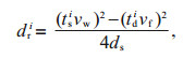
(2)where dri and xhi are the depth and horizontal offset of the ith hydrophone, respectively; tdi and tsi are the arrival times of the direct wave and sea surface reflection wave of the ith hydrophone picked from seismic records, respectively; vw is the average velocity of the whole water column in the survey line area; vf is the velocity of the deep part of the water column near the seafloor, as measured by the CTD; and ds is the depth of the source, measured by the depth sensor. Seismic records of sea surface reflection waves in the Shenhu and Qiongdongnan areas are shown in Fig. 4a & c, respectively, and the hydrophone positions calculated by Eqs.1 & 2 (e.g., vw=1 484.5 m/s, vf=1 483.7 m/s) are shown in Fig. 4b & d. However, the results show that when vw is 1 484.5 m/s, the extension line (green dashed line in Fig. 4b & d) of the towing hydrophone array does not pass the shot point, which is inconsistent with the actual situation. Therefore, the positioning result must be corrected by adjusting the velocity of sea water.

|
| Fig.4 Examples of seismic records of sea surface reflection waves and travel-time positioning results a. seismic records of the sea surface reflection wave in the Shenhu area; b. travel-time positioning results of Fig. 4a; c. seismic records of the sea surface reflection wave in the Qiongdongnan area; d. travel-time positioning results of Fig. 4c. |
Because the weight of the digital transmission packet (Fig. 1, A) connecting each working section is made of stainless steel (length: 0.25 m, diameter: 0.20 m, and weight: 1.85 kg), the gravity of the connection point is greater than the buoyancy, and as a result, the streamer is W-shaped, so the shape and position of the front section (minimum offset) cannot be accurately determined (Wei et al., 2020; Zhu et al., 2020a, b). By installing the buoyancy block (K2, as shown in Fig. 1), the hydrophone streamer appears as a curve or straight line during towing. Based on this phenomenon, we use the following process to correct the positioning results. First, the depth of the initial positioning hydrophone is fitted the polynomial curve fitting method (curve fitting tool of MATLAB, MathWorks, Inc.), which is expressed by the following equation:
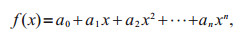 (3)
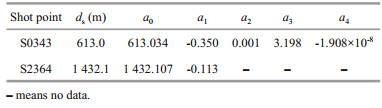
(3)where a0, a1, a2, …, an are the coefficients of the polynomial. Fourth order polynomial fitting is the best and most stable for the curve shape of streamer, and linear fitting is used for the straight. Then, if the curve is at the position of "curve a" as shown in Fig. 5, the sea water velocity of positioning should be increased until a0≈ds; conversely, if the curve is at the position of "curve b" the sea water velocity of positioning should be decreased. The coefficients of the fitting curves of S0343 and S2346, and the depth of the shot point are shown in Table 1, where a0 is very close to ds. The final corrected positioning results in which the extension line (green dashed line) of the towed hydrophone streamer passes the shot point are shown in Fig. 6, and the optimal positioning sea water velocities of S0343 and S2346 are 1 490.865 m/s and 1 485.217 m/s, respectively. The positioning result of the towing hydrophone array has been corrected.

|
| Fig.5 Diagram of polynomial curve fitting correction |

|
| Fig.6 Examples of the polynomial curve fitting method correcting the travel-time positioning result a. polynomial curve fitting method correcting the travel time positioning result of shot S0343; b. polynomial curve fitting method correcting the travel time positioning result of shot S2364. Green dashed lines show the final corrected positioning results in which the extension line of the towed hydrophone streamer passes the shot point. V is the submarine sound velocity. |
By installing a buoyancy block at the joint, the shape of the streamer presents a curve or straight line shape, so that the error caused by inaccurate velocity can be corrected by polynomial curve fitting. In addition, the results of polynomial curver fitting solve the problem that the streamer shape is not smooth due to phase distortion of sea-surface reflection waves.
3.2 Processing workflowA total of 220 shots of Line 1 in the Qiongdongnan area are used for data processing examples, the geometry is established with positioning data, and the common mid-point (CMP) bin is 1.5 m. The data processing workflow is shown in Fig. 7. The geometry and configuration were set up using positioning results. Some of the methods used in this processing workflow are the same as those used in traditional marine surface towed seismic data processing, such as band pass filtering, FK filtering (removing linear noise generated by the towed ship propeller), velocity analysis, normal moveout correction and imaging. Then, the float datum setting, residual static, residual phase moveout correction and seafloor time correction, which are different from conventional marine seismic data processing, are emphasized in the following sections.

|
| Fig.7 The data-processing flow chart for Kuiyang-ST2000 system seismic data |
The sea level is set as a fixed datum in the process of conventional sea surface seismic data (3-D or 2-D) processing, while the depths of the source and hydrophone changes due to the special operation mode of the deep-towed system; in other words, the shot point and towed hydrophone streamer need to be at a certain height from the seafloor or the towed speed is not stable. Referring to the datum setting as land complex surface data processing, the shot point and hydrophone point are placed on a relatively smooth float datum, as shown in Fig. 8.

|
| Fig.8 Diagram of the float datum of the deep-towed system C: fixed datum; S: trajectory of the tow body; F: float datum; f1–f4: datum of the CMP gather. |
A conventional static t(j) can be calculated by using the following equation (Yilmaz, 2001):
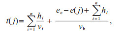 (4)
(4)where e(j) is the depth of shot j; hi and vi are the thickness and velocity of each low-velocity layer, respectively; n is the number of low-velocity layers; vb is the replacement velocity; and ec is the elevation of the fixed datum. The surface consistency statics of the shot point and receiving point relative to the fixed datum are calculated by using Eq.4. Then, the statics t(k) between the float datum and fixed datum can be calculated by using the following equation:
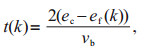 (5)
(5)where k is the number of the CMP and ef(k) is the elevation of the float datum. If the complex deep-towed trajectory is regarded as a complex surface, the float datum correction of deep-towed data can be calculated by Eqs.4–5. Then, e(j) is the depth of shot j, hi and vi are the thickness and velocity of sea water (between the deep-towed system and the seafloor) (e.g., 1 481.9 m/s, as measured by CTD), and n is 1. vb is the average velocity of the layers below the seafloor (e.g., 1 610 m/s). The float datum of deep-towed data ef(k) is determined by using a smooth shot point depth, and the smooth radius is 158 m of the offset length. Figure 9 shows the float datum established for 220 shot data points of survey Line 1. The velocity distributions without and with a static float datum are shown in Fig. 10a–c and Fig. 11a–c, respectively. By comparison, the focusing effect of the energy group of the velocity spectrum with a static float datum is very accurate, which is beneficial to the fine velocity analysis.

|
| Fig.9 Example of the float datum of Line 1 based on the shot depth |

|
| Fig.10 Examples of velocity semblance panels without float datum time moveout correction a. velocity semblance panel of CMP200; b. velocity semblance panel of CMP400; c. velocity semblance panel of CMP600. |

|
| Fig.11 Examples of velocity semblance panels after float datum time moveout correction a. velocity semblance panel of CMP200; b. velocity semblance panel of CMP400; c. velocity semblance panel of CMP600. |
Residual static correction based on surface consistency or nonsurface consistency require fixed source and receiver positions, which is not applicable to marine seismic data (Gutowski et al., 2002). For deep-towed seismic data, first, the source and hydrophone move continuously, and the distance of each shot position depends on the ship velocity. Second, the depth of the source and hydrophone is varied. Therefore, the residual static correction method is not suitable for high-frequency deep-towed data, so the following steps are used to correct the moveout after the first normal moveout correction (NMO).
Step 1: Calculate the time difference of the seafloor first arrival wave between each channel of the CMP gather and others by the cross-correlation method and sum these time differences.
Step 2: Select the trace with the smallest sum calculated in step 1 as the reference trace and calculate the time difference between the seafloor first arrival wave travel-time of other channels and the reference trace.
Step 3: Use the time calculated in step 2 to correct the moveout of the CMP gather after NMO.
Step 4: Use the float datum depth df to calculate time tf (tf=df/vw, where vw is the average velocity of seawater) and calculate the time between tf and the time of the seafloor first arrival wave in the CMP gather.
Step 5: Use the time calculated in step 4 to correct the moveout of the CMP gather and then sort the stack in the CMP.
The moveout within the CMP gather (CMP151, CMP161, and CMP171) exists after the first NMO, as shown in Fig. 12a–c. After the correction in step 3, the correction effect is shown in Fig. 13a–c, and the moveout has basically been corrected. The partial stack profile without residual moveout correction is shown in Fig. 14a, and that with residual moveout correction in step 3 is shown in Fig. 14b, while the phase is discontinuous. After the correction in step 5, the effect is shown in Fig. 14c: the discontinuity on the stack profile is basically eliminated. Furthermore, the corrected CMP gather is processed with the inverse NMO method using the velocity function of the first NMO, and then interactive velocity analysis is performed. Some examples of velocity semblance panels are shown in Fig. 15a–c. Compared with Fig. 11, the semblance energy is improved, which can further improve the accuracy of the velocity analysis.

|
| Fig.12 Examples of CMP gathers after normal moveout correction a. gather of CMP151; b. gather of CMP161; c. gather of CMP171. |

|
| Fig.13 Examples of CMP gathers after step 3 time moveout correction a. gather of CMP151; b. gather of CMP161; c. gather of CMP171. |

|
| Fig.14 Comparison of the partial CMP stack profile after and without step 3, step 5 time moveout correction a. CMP stack profile without residual moveout correction; b. CMP stack profile after step 3 and without step 5 moveout correction; c. CMP stack profile after step 5 moveout correction. |

After residual moveout correction, there is nonconsistent moveout in the CMP gather because the drag trajectory changes so dramatically, as shown in Fig. 12a–c. However, residual and surface consistency statistical methods cannot be used to solve these problems. Therefore, the phase-based moveout correction method is used to correct inconsistent moveout (Lichman, 1999). The phasebased moveout correction method is described as follows. The time sequence s(t) is as follows:
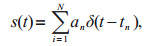 (6)
(6)where N is the number of seismic data samples; an and tn are the seismic amplitude and the arrival time of n sample numbers, respectively; and δ(t–tn) is the delta function. Then, the amplitude spectrum and phase spectrum of the time sequence s(t) are described by the following equation:
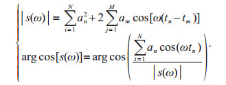 (7)
(7)The result shown in Eq.7 is that arrival time information is included in the phase spectrum of s(t). Therefore, the purpose of moveout can be corrected by changing the phase spectrum. The phase-based moveout correction can be represented by the following equation:
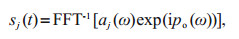 (8)
(8)where j is the trace number within the CMP gather, FFT-1 is an inverse fast Fourier transform (FFT) procedure, ω is the frequency, aj(ω) is the amplitude spectrum of trace number j, and po(ω) is the phase spectrum that substitutes for the phase spectrum of the original trace. Theoretically, po(ω) should be equal to the phase spectrum of the minimum offset trace. However, it is very common that the signal quality of near-offset traces is not very good. To minimize the influence of the minimum-offset traces and to maximize the signal-to-noise ratio, traces 1 to 4 or 1 to 6 of the stacked CMP gather are used as reference traces to obtain po(ω). Figure 16a–c shows the CMP gather after residual moveout correction, and the same CMP gather after phase-based moveout correction is shown in Fig. 16d–f. The nonconsistent moveout on the CMP gather has been corrected, and the signal-to-noise ratio and resolution have been improved, as shown in Fig. 17b, compared with the uncorrected (Fig. 17a), especially within the yellow circles, the resolution has been significantly improved.

|
| Fig.16 CMP gather before and after applying the phase-based moveout correction method a–c. CMP gather without phase-based moveout correction; d–f. CMP gather after phase-based moveout correction. |

|
| Fig.17 CMP stack profile before and after applying the phase-based moveout correction method a. stack profile without phase-based moveout correction; b. stack profile after phase-based moveout correction. |
After moveout correction, the CMP stack or migration methods of conventional seismic data processing can be used for deep-towed data. The profile that uses Kirchhoff prestack migration (Yilmaz, 2001) on the float datum is shown in Fig. 18a & c. However, because the float datum is irrelevant to the seafloor, the profile has not been corrected from the float datum to the fixed datum. The seafloor time tfloor is used to correct the migration profile as follows:
 (9)
(9)

|
| Fig.18 Example of a migration profile before and after seafloor time correction a, c. migration profile without seafloor time correction. The time range in (a) is 125-200 ms, and that in (c) is 200-320 ms; b, d. migration profile with seafloor time correction. The time range in (b) is 2.035-2.100 s, and that in (d) is 2.100-2.220 s. In the red box position, there was no pockmark structure before correction, but it appeared after correction. |
where tfloatdatum is the time of the float datum; dcmpi is the ith CMP depth of the seafloor, as summed by the depth (measured by depth sensor) and the height (measured by altimeter) of the towed body within the survey line; and the results are smoothed and linearly interpolated. vw is the average velocity of the whole water column in the survey line area (e.g., 1 484.5 m/s). In addition, if there are other high-resolution data for the seafloor in the study area, such as sub-SBP and multibeam bathymetry data, the stack or migration profile can be corrected to the seafloor time of these data. The profile after seafloor time correction is shown in Fig. 18b & d, which is more consistent with the true structural feature of the strata below the seabed. In particular, in the red box position, there was no pockmark structure before correction, but it appeared after correction.
4 RESULT AND DISCUSSIONThe Kuiyang-ST2000 system was used to collect data in gas hydrate exploration areas in the Qiongdongnan area (Line 1) and Shenhu area (Line 2) in the South China Sea. The positions of the two survey lines are shown in Fig. 19. Line 1 is in the Qiongdongnan Basin and has a water depth range from 1 400 to 1 520 m, and Line 2 is in the Zhujiang (Pearl) River Mouth Basin and has a water depth range from 800 to 1 500 m. The towing speed of the deep-towed system was 3 knots (1.5 m/s). The source was shot at equal spacing (6.25 m), with a minimum offset of 12.5 m, and the maximum fold was 12 times. The data sampling interval was 0.125 ms, and the record length was 3 s.

|
| Fig.19 Bathymetric map of the study areas in the South China Sea The red line is the Kuiyang-ST2000 survey Line 1 in the Qiongdongnan area of the South China Sea, and the yellow line is the Kuiyang-ST2000 survey Line 2 in the Shenhu area of the South China Sea. |
The partial CMP stack profile of Line 1 is shown in Fig. 20a. Compared with the same position on the conventional 3-D seismic line profile (Fig. 20b), there are two small pockmarks on the deep-towed seismic profile, but the 3-D seismic profile is not shown. The lateral resolution (first Fresnel zone: better than 8 m) and the vertical resolution (better than 0.5 m) of the deep-towed data is higher than that of the 3-D seismic data. In the deep-towed seismic profile, there are several sets of mass transport deposits (MTDs), while in the 3-D seismic profile, they are shown as only one layer. Furthermore, small structural units, such as gas chimneys, pipes and, small faults, can be found in deep-towed seismic profiles, which are difficult to interpret in 3-D seismic profiles. The results show that the vertical and lateral resolutions of the deep-towed high-resolution seismic data are higher than those of the 3-D seismic data. The partial profile of Line 2 is shown in Fig. 21a. Compared with the conventional 2-D seismic profile of the adjacent survey line (Fig. 21b) (Xu et al., 2010), there is a small pockmark in the deep-towed seismic profile, and a gas chimney can be interpreted. The BSR is also interpreted in the deep-towed seismic profile, and the distribution of the BSR can be clearly described. Furthermore, compared with the SBP line (1 800–5 000 Hz) (Li et al., 2011), as shown in Fig. 22, the results show that the average acoustic penetration of the SBP profile (Fig. 22a) is approximately 100 ms (two-way time), and the signal-to-noise ratio of the profile is lower. Obviously, Fig. 22b shows that the average acoustic penetration of the deep-towed profile (part of Line 2) is 400 ms (two-way time), and fine layering of slope sediments, blanking zones, small faults (red lines), and BSRs can be identified clearly.

|
| Fig.20 Comparison between deep-towed seismic profiles and sea surface 3-D seismic profiles in the Qiongdongnan area, South China Sea a. deep-towed profile (part of Line 1); b. seismic line profile extracted from a 3-D cube. |

|
| Fig.21 Comparison between the deep-towed seismic profile and the surface 2-D seismic profile in the Shenhu area, South China Sea a. deep-towed profile (part of Line 2); b. surface 2-D line seismic profile (modified from Xu et al. (2010)). |

|
| Fig.22 Comparison between deep-towed seismic profile and subbottom profile data in the Shenhu area, South China Sea a. subbottom profiler line (1 800-5 000 Hz) (modified from Li et al. (2011)) showing that the average acoustic penetration is approximately 100 ms (two-way time) and showing the lower signal-to-noise ratio of the profile; b. deep-towed profile (part of Line 2). |
The resolution capability of the Kuiyang-ST2000 deep-towed high-resolution multichannel seismic system is demonstrated in this paper. Currently, the system is capable of finely investigating small structures hundreds of meters below the seabed in deep water, but the data require fine processing. In terms of positioning, considering that the hydrophone streamer is characterized by smooth curves or straight lines in towing, the travel-time positioning results of the towed hydrophone streamer have been modified by the polynomial curve fitting method, basically meeting the requirements of positioning accuracy for deep-towed data processing. In terms of data processing, firstly, the static float datum method was used, and the energy group of the velocity semblance after correction is well focused, which is beneficial to interactive velocity analysis. The residual time moveout after NMO is corrected by using the autocorrelation statistics of the first arrival time of the seafloor, the correction value is applied to the common source gather (CSG) set, and the velocity semblance is further improved. Then, phase-based moveout correction is used to correct the inconsistent time moveout in the CMP gather after the above time moveout correction processing, and the resolution of the stack profile after correction is improved. Finally, the seafloor smoothing time is corrected for the stacked or migration profile, and the corrected profile can indicate the structural morphology of the seabed and the strata below. We obtained high-resolution imaging profiles (vertical resolution better than 0.5 m and lateral resolution better than 8 m) of two survey lines in Qiongdongnan and Shenhu waters in the South China Sea. Compared with the conventional surface-towed 3-D and 2-D seismic data (vertical resolution less than 3.5 m and lateral resolution less than 100 m), the results show that the deep-towed data can identify small geological structures, such as small faults, gas chimneys, pockmarks, pipes, and MTDs. In addition, the penetration capability and signal-to-noise ratio of the deep-towed profile are better than those of the subbottom profile data. Therefore, Kuiyang-ST2000 can meet the needs of the exploration and development of natural gas hydrate in the South China Sea and other areas, as well as the understanding of shallow structures below the seafloor and evaluation of the potential geohazards in major marine engineering construction in deep water. However, there are still some shortcomings in this paper. At present, it takes a great deal of time to make the fitting curve pass through the shot point by manually changing the sea water velocity. In addition, because the phase-based moveout method does not have the correction time output, the time correction cannot be applied to the CSG gathers, and as a result, migration imaging may not be sufficient.
6 DATA AVAILABILITY STATEMENTAll data generated and/or analyzed during this study are not availiable due to commercial restrictions.
Asakawa E, Mizohata S, Inamori T et al. 2009. High resolution, deep-tow seismic survey to investigate methane hydrate-bearing sediments, Nankai Trough, Offshore Japan. In: Oceans 2009-EUROPE. IEEE, Bremen, Germany. p. 1-8.
|
Byrd R H, Schnabel R B, Shultz G A. 1988. Approximate solution of the trust region problem by minimization over two-dimensional subspaces. Mathematical Programming, 40(1-3): 247-263.
DOI:10.1007/BF01580735 |
Chapman N R, Gettrust J F, Walia R, et al. 2002. High-resolution, deep-towed, multichannel seismic survey of deep-sea gas hydrates off western Canada. Geophysics, 67(4): 1038-1047.
DOI:10.1190/1.1500364 |
Colin F, Ker S, Marsset B. 2020a. Fine-scale velocity distribution revealed by datuming of very-high-resolution deep-towed seismic data: example of a shallow-gas system from the western Black Sea. Geophysics, 85(5): B181-B192.
DOI:10.1190/geo2019-0686.1 |
Colin F, Ker S, Riboulot V, et al. 2020b. Irregular BSR: evidence of an ongoing reequilibrium of a gas hydrate system. Geophysical Research Letters, 47(20): e2020GL089906.
DOI:10.1029/2020GL089906 |
Gutowski M, Breitzke M, Spieß V. 2002. Fast static correction methods for high-frequency multichannel marine seismic reflection data: a high-resolution seismic study of channel-levee systems on the Bengal Fan. Marine Geophysical Researches, 23(1): 57-75.
DOI:10.1023/A:1021240415963 |
He T, Spence G D, Wood W T, et al. 2009. Imaging a hydrate-related cold vent offshore Vancouver Island from deep-towed multichannel seismic data. Geophysics, 74(2): B23-B36.
DOI:10.1190/1.3072620 |
Ker S, Marsset B, Garziglia S, et al. 2010. High-resolution seismic imaging in deep sea from a joint deep-towed/OBH reflection experiment: application to a mass transport complex offshore Nigeria. Geophysical Journal International, 182(3): 1524-1542.
DOI:10.1111/j.1365-246X.2010.04700.x |
Ker S, Gonidec Y L, Marsset B, et al. 2014. Fine-scale gas distribution in marine sediments assessed from deep-towed seismic data. Geophysical Journal International, 196(3): 1466-1470.
DOI:10.1093/gji/ggt497 |
Kong F D, He T, Spence G D. 2012. Application of deep-towed multichannel seismic system for gas hydrate on mid-slope of northern Cascadia margin. Science China Earth Sciences, 55(5): 758-769.
DOI:10.1007/s11430-012-4377-4 |
Leon P, Ker S, Gall Y L et al. 2009. SYSIF a new seismic tool for near bottom very high resolution profiling in deep water. In: Oceans 2009-EUROPE. IEEE, Bremen, Germany. p. 1-5.
|
Li S J, Chu F Y, Fang Y X, et al. 2011. Associated interpretation of sub-bottom and single-channel seismic profiles from Shenhu Area in the north slope of South China Sea—haracteristic of gas hydrate sediment. Advanced Materials Research, 217-218: 1430-1437.
DOI:10.4028/www.scientific.net/AMR.217-218.1430 |
Lichman E. 1999. Automated phase-based moveout correction. In: SEG Technical Program Expanded Abstracts 1999. Houston. p. 1150-1153, https://doi.org/10.1190/1.1820706.
|
Marsset B, Ker S, Thomas Y, et al. 2018. Deep-towed high resolution seismic imaging Ⅱ: Determination of P-wave velocity distribution. Deep Sea Research Part Ⅰ: Oceanographic Research Papers, 132: 29-36.
|
Marsset B, Menut E, Ker S, et al. 2014. Deep-towed High Resolution multichannel seismic imaging. Deep Sea Research Part Ⅰ: Oceanographic Research Papers, 93: 83-90.
DOI:10.1016/j.dsr.2014.07.013 |
Marsset T, Marsset B, Ker S, et al. 2010. High and very high resolution deep-towed seismic system: Performance and examples from deep water Geohazard studies. Deep Sea Research Part Ⅰ: Oceanographic Research Papers, 57(4): 628-637.
DOI:10.1016/j.dsr.2010.01.001 |
Riboulot V, Sultan N, Imbert P, et al. 2016. Initiation of gas-hydrate pockmark in deep-water Nigeria: Geo-mechanical analysis and modelling. Earth and Planetary Science Letters, 434: 252-263.
DOI:10.1016/j.epsl.2015.11.047 |
Rowe M M, Gettrust J F. 1993. Faulted structure of the bottom simulating reflector on the Blake Ridge, western North Atlantic. Geology, 21(9): 833-836.
DOI:10.1130/0091-7613(1993)021<0833:FSOTBS>2.3.CO;2 |
Walia R, Hannay D. 1999. Source and receiver geometry corrections for deep towed multichannel seismic data. Geophysical Research Letters, 26(13): 1993-1996.
DOI:10.1029/1999GL900402 |
Ward P, Asakawa E, Shimizu S. 2004. High resolution, deep-tow seismic survey to investigate the methane hydrate stability zone in the Nankai Trough. Resource Geology, 54(1): 115-124.
DOI:10.1111/j.1751-3928.2004.tb00193.x |
Wei Z R, Pei Y L, Liu B H. 2020. A new deep-towed, multi-channel high-resolution seismic system and its preliminary application in the South China Sea. Oil Geophysical Prospecting, 55(5): 965-972.
(in Chinese with English abstract) DOI:10.13810/j.cnki.issn.1000-7210.2020.05.004 |
Xu H N, Yang S X, Zheng X D, et al. 2010. Seismic identification of gas hydrate and its distribution in Shenhu Area, South China Sea. Chinese Journal of Geophysics, 53(7): 1691-1698.
(in Chinese with English abstract) |
Yilmaz Ö 2001. Seismic Data Analysis: Processing, Inversion, and Interpretation of Seismic Data. Science of Exploration Geophysicists, Tulsa. p. 380-383, https://doi.org/10.1190/1.9781560801580.
|
Zhu X Q, Wang Y F, Yu K B, et al. 2020a. Dynamic analysis of deep-towed seismic array based on relative-velocity-element-frame. Ocean Engineering, 218: 108243.
DOI:10.1016/j.oceaneng.2020.108243 |
Zhu X Q, Wei Z R, Pei Y L, et al. 2020b. Dynamic modeling and position prediction of deep-towed seismic array. Journal of Shandong University (Engineering Science), 50(6): 9-16.
(in Chinese with English abstract) DOI:10.6040/j.issn.1672-3961.0.2020.084 |