 2023, Vol. 41
Institute of Oceanology, Chinese Academy of Sciences
Article Information
- LUO Yao, YIN Hang, LIU Qiang, LI Jingmin, LIU Shihua, GAO Wei, LI Rui, YANG Yi
- Tectonic boundaries in the South China Sea from aeromagnetic signature
- Journal of Oceanology and Limnology, 41(2): 550-561
- http://dx.doi.org/10.1007/s00343-022-2043-z
Article History
- Received Apr. 2, 2022
- accepted in principle May 9, 2022
- accepted for publication Jun. 23, 2022


The South China Sea (SCS), located in the south of China and between the Philippines to the east and Vietnam to the west, is one of the largest marginal seas in the western Pacific Ocean (Fig. 1). The SCS, surrounded by the Eurasia, Indo-Australia, and Pacific plates, provides insights into the interaction between the Pacific tectonic domain and the Tethyan tectonic domain (Sun et al., 2018). Nonetheless, the formation of the SCS remains uncertain and controversial, and various tectonic mechanisms have been proposed for its origin and evolution. These mechanisms involve the extrusion model of the Tibetan Plateau, which suggests that penetration of India into Asia has rotated and extruded to the southeast along the left-lateral Red River Fault, forming the opening of the SCS basin (e.g., Tapponnier et al., 1982; Briais et al., 1993; Leloup et al., 2001; Replumaz and Tapponnier, 2003). Another contrasting explanation is the extension in the SCS, including sea-floor spreading, within the continental rifting of the North Palawan block from the Asian mainland (e.g., Taylor and Hayes, 1980, 1983; Holloway, 1982). Lately, several tectonic models have merged elements of both the contrasting points mentioned above (Mazur et al., 2012). Despite the different patterns of evolution in the SCS, we believe that a significant evidence for its formation is the presence of magnetic anomalies in the oceanic SCS basin.

|
| Fig.1 Data source for the new compilated magnetic map in the SCS All geographical base maps for this article are from the Ministry of Natural Resources of the People's Republic of China (map review No. GS(2016)1663). |
In early surveys, magnetic anomalies play a decisive role in the geodynamics of the SCS, such as determining the ages and stages of seafloor spreading. The earliest contribution may be credited to Ben-Avraham and Uyeda (1973), they identified EW trending striped magnetic anomalies in the deep-sea basin of the SCS. Taylor and Hayes(1980, 1983) inferred that the opening of SCS in a roughly NS direction occurred between approximately 32 and 17 Ma from a set of closely spaced marine magnetic profiles. The following is a series of research on the evolution of the SCS based on magnetic records. However, the age and the spreading history of the SCS basin have long been controversial. For example, Briais et al. (1993) identified magnetic anomaly 5c and suggested that seafloor spreading ended at 16 Ma; Hsu et al. (2004) identified the oldest oceanic crust of the SCS (magnetic anomaly C17), implying the basin opened as early as 37 Ma. The main reasons for this controversy are the low accuracy of the early magnetic tracks and the atypical stripes in the SCS. Previous magnetic anomaly data from shipboard surveys acquired are over the past decades with low accuracy and resolution. As Li and Song (2012) pointed out, the limited number of magnetic tracks tend to be widely spaced, which brings a large margin of uncertainties in the study.
In recent years, the compilations of magnetic tracks via 2D re-interpolation grids became part of the interpretation that provides an overview of the magnetic field. Available grids data, such as the Magnetic Anomaly Map of East Asia (MAMEA) or 2-arc min resolution Earth Magnetic Anomaly Grid (EMAG2) (Geological Survey of Japan and AIST and Coordinating Committee for Coastal and Offshore Geoscience Programmes in East and Southeast Asia (CCOP), 2002; Maus et al., 2009; Meyer et al., 2017), were used to study the magnetic stripes and Curie-point depths in the SCS (e.g., Li and Song, 2012; Li et al., 2017; Wang et al., 2020). The re-interpolation of the magnetic tracks provides a 2D grid map, whereas parts of the magnetic field details were lost or erroneous in the map due to the far-spaced track lines. However, the map displays a clearer view of completely obscured rocks, allowing much finer divisions of provinces (Pilkington et al. 2000). For example, Dai (2018) divides the SCS into eight districts with EMAG2 data, considering different geological formations.
In reality, little attention has been paid to the overview pattern of anomalies compared with the magnetic stripes in the basin zone due to the lack of high-resolution magnetic data in the SCS. As the compilations of aeromagnetic surveys are extended to the sea area, the continuous magnetic data stitch the isolated interpretation together, thus providing new perspectives on the geologic structure and improving the geological mapping in the mainland and the SCS. This paper will focus on the importance of the distribution of magnetic anomalies in the SCS. Knowledge of magnetic field patterns is known to help improve understanding of the tectonic units and crystalline basement rocks. In this paper, we present the delineating areas of magnetic anomalies having similar characteristics in the SCS that isolate areas of crust having similar structural character and possibly history. To achieve this, we discuss the magnetic boundaries of the SCS with the magnetic data from the new compilations (Yin et al., 2015a, 2018) based on aeromagnetic surveys that provide a macroscopic distribution of the magnetic field in the SCS.
2 MAGNETIC DATASince the 1950s, the United States conducted marine geophysical and aeromagnetic surveys (Project Magnet airborne data of the Naval Research Lab) in the SCS and its surrounding waters. China's marine geophysical surveys, including aeromagnetic surveys in the SCS, began in the 1970s. A variety of factors determine the importance of marine research to China: the development of the marine economy, the protection of the marine environment, the protection of national maritime rights and interests, and the resolution of maritime disputes. Therefore, the development of the marine geology and geophysics program is of great significance in reality. In recent years, large-scale aeromagnetic surveys have been carried out in the SCS, and it has become possible to compile a magnetic map of the SCS from aeromagnetic and ship-track data. In this study, the magnetic anomaly data (Yin et al., 2015a, b, 2018) from the compilation of the magnetic anomaly map that covers the mainland of China, offshore, and adjacent areas were used, and it is a significant update of the compilated map of airborne and ship-track magnetic measurements. Unlike previous ones with missing data in the SCS, the new magnetic map covers all areas of existing surveys, as interpolated data is used for unmeasured areas.
Figure 1 shows the data sources of our study areas. The areas cover the SCS and its adjacent areas, from 0° to 26°N and from 105.5°E to 122°E, and most of the magnetic data were from the high-accuracy aeromagnetic surveys collected in recent years. Over map, preexisting survey grids derived from airborne and shipboard surveys were merged using the toolkit of Oasis Montaj GridKnitTM. The airborne data are from Aerogephysical Survey, China Geological Survey, and the ship-track date are from GETECH, Leeds, UK. The remaining is from MAMEA (Geological Survey of Japan and AIST and Coordinating Committee for Coastal and Offshore Geoscience Programmes in East and Southeast Asia (CCOP), 2002) or EMAG2 data (Maus et al., 2009). All individual grids are continued to a surface level and merged representing magnetic anomalies at 1-km altitude above the sea or ground level in 5-km resolution. Figure 2 displays the magnetic map of the SCS and adjacent areas. We compare the final magnetic grid with MAMEA and EMAG2 grids, and Fig. 3 shows the maps of the MAMEA and EMAG2 data. Although the MAMEA grid shows details of magnetic anomalies due to observations at sea level, in reality, the MAMEA and EMAG2 data are from the same source in the SCS, part of which was from Guangzhou Marine Geological Survey MGMR, China. Unlike other data, Fig. 2, in the SCS, is mainly from airborne surveys with a minimum line spacing of 20 km in the NS direction and tie-line spacing of 100 km in the EW direction. By contrast, the previous ship-track magnetic data has low accuracy, e.g., MAMEA grid data (Fig. 3a) reflects low signal-to-noise ratio (S/N) magnetic anomalies. In reality, the early magnetic anomaly maps of the SCS compiled by the Guangzhou Marine Geological Survey MGMR could not perform on the grid but profiles (Liu, 1992). Hence, the airborne data improved data resolution compared to ship-track magnetic data, providing a high S/N magnetic data of the SCS. In summary, the new compilation of magnetic fields major from the aeromagnetic surveys shows the connection between the magnetic fields of the Chinese mainland and the SCS, providing insight into the subsurface structure and composition of the crust.

|
| Fig.2 New magnetic map of the SCS and adjacent areas |

|
| Fig.3 Magnetic maps of the MAMEA (a) and EMAG2 (b) data |
As shown in Figs. 2–3, as a whole, a large number of striped magnetic anomalies exist in the SCS, and some negative and positive magnetic anomaly zones also exist. Figures 2–3 clearly show the linear trend of the magnetic anomalies. To clearly show the trends, we manually track the direction and scales of magnetic anomalies. In Fig. 4, the positive anomaly of more than 50 nT is shown as the black line, and the length is usually more than 50 km. For negative anomalies below -80 nT, the main distribution areas are represented with the green-filled area. Since the SCS lies at low geomagnetic latitudes, if we ignore the remanent magnetization, the magnetic anomalies are generated by the horizontal magnetization. As the orientation of the core field is roughly horizontal along the NS direction, the boundary will reinforce the characteristics of the magnetic source along the EW direction, and the magnetic anomalies in Fig. 4 show a trend in the EW direction. Coincidentally, the magnetic stripes are also nearly in the EW direction in the SCS. Although the magnetic stripes in the SCS reflect residual magnetism due to the spreading of mid-ocean ridges in the NS direction, the characteristics of the stripes in the EW direction will be reinforced by the present core field.

|
| Fig.4 Sketch of magnetic anomaly in the SCS |
In contrast to magnetic sources extending in the EW direction, the magnetic sources that extend in the NS direction, e.g., the Western Margin Fault (WMF or East Vietnam Fault, NS direction), reflects the string of pearls-like anomalies with a linear trend. As shown in Fig. 4, we have also connected the pearl-like magnetic anomalies with black lines to represent the linear trend of these magnetic sources in the NS direction. These pearl-like magnetic anomalies show the fault systems separating the SCS and surrounding blocks, including the Southern Margin Fracture, roughly along the U-shaped line (Li et al., 2022) distinguishing the anomalies of the SCS from the surrounding magnetic anomalies.
3.2 Geological structureAs a wedge-shaped block, the SCS lies at the intersections of the Eurasian plate, Philippine Sea plate, and Indo-Australian plate. We know that there are large fault structures in the SCS, some of which can be identified by magnetic anomaly data, and others are more difficult to be identified due to low magnetism. Since there are numerous magnetic strips on the magnetic anomaly map and strong remanent magnetization, pseudo gravity, Euler deconvolution, and the directional derivative are adopted to identify some of the fault structures (Figs. 5–7).

|
| Fig.5 The horizontal gradient of pseudo-gravity anomaly |

|
| Fig.6 The solution of Euler deconvolution with the base map of magnetic data |

|
| Fig.7 Result of the directional derivative of magnetic anomaly (I=45°, D=90°) (a) and the Euler solution (b) with the base map of pseudo gravity The fault structures are after Yin et al. (2015b, 2018). The white line is the fault and the yellow circle is the location of the Euler deconvolution. |
Pseudo gravity is a gravity-like anomaly that implies the constant magnetization assumption based on Poisson's relationship (Baranov, 1957) as a linear filter usually applied in the Fourier domain. Pseudo gravity is adopted to eliminate the target distortion due to the obliquity of the core field and determine the edges of magnetic bodies (Blkely et al., 1986). The maximum horizontal gravity gradients are close to the source edge, and the maximum pseudo gravity gradients may overlie the edges of causative magnetic bodies. It has been successfully used to enhance the boundary of bodies and explain the crustal structure (Ates et al., 2012; Aslan et al., 2013; Aydemir et al., 2015; Bilim et al., 2016, 2021). The technique of pseudo gravity was applied for our magnetic data. Before translating the magnetic data to pseudo gravity, we assumed that the scenario of a total-field anomaly is produced only by induced magnetization. Similar to the reduction to the pole, when translating the magnetic to pseudo gravity, the variation of both magnetic inclination and declination should be considered (Arkani-Hamed, 1988, 2007); while at low latitudes, a suppression filter was routinely applied (Yao et al., 2003).
Figure 5 shows the gradient of pseudo gravity of the magnetic data. Though the influence of magnetic remanence is not considered, to some extent, the pseudo-gravity gradient data can also reflect the distribution of underground magnetic bodies. In the area with low precision data (or interpolation data), e.g., 110°E–116°E, 0°–6°N, the gradient of pseudo gravity is meaningless.
3.2.2 Euler deconvolutionEuler deconvolution based on the Euler equation is commonly applied to magnetic and gravity interpretation. Without prior information, it can also obtain reliable locations. Reid et al. (1990) applied the method to gridded data, and then the method has been widely used to estimate the crustal thickness, enhance the geology body edge, and locate the position of the faults and minerals. In the processing, we used the Euler deconvolution method (Stavrev, 1997), and the structural index was treated as an unknown parameter. The window size is 11×11 (~10 km×10 km), and the solutions with lower uncertainty are ignored. Figure 6 shows the results while the circle represents the horizontal solutions and the color represents the depth solutions.
According to the results of Euler deconvolution and pseudo gravity, combined with the previous research results (Yin et al., 2015b), we draw the main fault structures (white line) distribution in the SCS in Fig. 7. Overall, the U-shaped line wraps the structures in the SCS region, which is similar to that mentioned before; that is the anomalies of magnetic data in the SCS are clearly different from those in the surrounding areas, and the dividing lines are roughly distributed along the U-shaped line. The U-shaped lines approximately delineate the SCS tectonic domain from the surrounding blocks. To verify this phenomenon, magnetic data of the SCS are processed further.
3.3 Texture analysisIn this section, we will discuss the tilt derivatives of the magnetic anomalies and the texture of the magnetic anomalies that can be used to divide the magnetic anomaly field. In practice, we should perform the processing of magnetic anomaly via reduction to the pole before calculating the texture of the magnetic data. However, the reduction processing for the SCS magnetic data faces the difficulty that the directions of the core field change with the latitudes at low latitudes. We need the operation of differential reduction to the pole at the magnetic equator (Arkani-Hamed, 1988, 2007). In addition, we need to consider the remanent magnetic effects of magnetic anomalies in the SCS, which is another difficulty. The residual magnetism in the SCS can exceed the induced magnetic anomaly, whereas we do not take the preprocessing of reduction to the pole. To reduce the effects of horizontal magnetization at low latitudes, here, we calculated the tilt derivative of the magnetic anomaly grid.
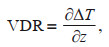
The tilt derivatives (TDR) of the magnetic anomaly are useful for mapping shallow basement structures and mineral exploration targets (Miller and Singh, 1994; Verduzc et al., 2004), which is defined as:
 (1)
(1)where VDR and THDR are the first vertical and total horizontal derivatives, respectively, of the total magnetic intensity anomaly ΔT, i.e., :
 (2)
(2)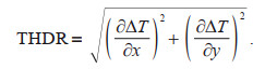 (3)
(3)Thus, the tilt derivatives are the angles of the gradient vector, ranging from -180° to 180°. Here, the tilt derivative is used as a texture for characterizing shallow magnetic anomalies in the SCS.
Compared with the total magnetic intensity, the tilt derivative reflects more details of the normalized texture due to the use of the angle. Figure 8 shows the tilt derivative map of the SCS. We can see that the tilt derivative map shows a more detailed but homogeneous texture than the original magnetic anomaly that reflects the shallow geological information. We could also interpret the characterization of the tilted derivative map in the representation of Fig. 8, but time-consuming, as this texture is more complex and denser than the magnetic anomaly map. Hence, we use the segmentation texture method instead of manual interpretation. Here, we adopted the segmentation based on the Local Binary Pattern (LBP) (Li and Staunton, 2008) to classify the tilt derivative map (Fig. 8) into 6 clusters, and the segmentation result is shown in Fig. 9.

|
| Fig.8 The texture of tilt derivative map |

|
| Fig.9 Texture segmentation result for Fig. 8 Different coloured blocks indicate different classifications.The dark blue line is the 1948s U-shaped line. |
According to the results of the texture segmentation, we can see that the SCS consists of two major classifications, the yellow and orange clusters in Fig. 9, which are similar to the Sulu-Sulawesi domain. The similarity between the SCS and the Sulu-Sulawesi Seas shown in Fig. 9 is not surprising due to the nature of the magnetic field that provides evidence of the magnetic stripes. Thus, the yellow blocks in Fig. 9 mainly reflect the magnetic characteristics of the SCS basin, and the orange blocks reflect the margin, which consists of major sedimentary basins of the SCS with hydrocarbon potential. The classification of purple and blue blocks reflects another feature of the magnetic anomaly. The purple block is the transition area to the blue block where the magnetic field data are spurious by interpolation due to unexplored area.
3.4 Interpreted domainsHere we have drawn an approximate U-shaped line, i.e., the dark blue line from the historical SCS maps (Tang et al., 2018; Luo et al, 2019; Li et al., 2022) as shown in Fig. 9. We can deduce that the dividing line between the green color cluster and the orange cluster is an approximately U-shaped line that corresponds well with the interpretation of the faults as shown in Fig. 7. Although the patterns of magnetic anomaly distribution shown in Fig. 9 is a simplistic result, it illustrates one of the most significant interpreted domains that separate the magnetic anomalies in the SCS from those generated by the surrounding blocks, approximately along the U-shaped line (dark blue line shown in Fig. 9). The division of the domain is the basis for the interpretation of magnetic anomalies. Combined with the result of texture segmentation, the distribution of the faults, and the magnetic data, we have reason to believe that the U-shaped line is an important geological and geophysical boundary (Fig. 10). Recently, Yin and Zhou (2018) and Zhang et al. (2017) divided the interpreted domain using the compilation map of magnetic anomalies in the SCS and adjacent areas. These interpretations of the magnetic domains are not only based on magnetic anomalies but also refer to other geological information. Here we combined the previous results and divided the SCS magnetic domain based on anomaly trend, texture, and amplitude. Figure 10 shows the delineated areas of the magnetic anomaly in the SCS. As Fig. 10 shows, the major interpreted domains consist of the South China domain, the SCS domain, and the surrounding domains.

|
| Fig.10 Interpreted domains of magnetic anomaly in the SCS Modified from Yin et al., 2015b, 2018. The green line is the interpreted domain boundary and the dark blue line is the 1948s U-shaped line. |
The South China domain could be divided into two subdomains, i.e., the Southeast Coast subdomain and the Yunnan-Guizhou-Guangxi subdomain. The SCS domain is divided from the South China domain by a giant belt of the magnetic anomaly along with the Dongsha Islands to Xisha Trough. The delineation of the SCS tectonic domain here is consistent with previous results, but the main difference is the northern boundary of the SCS. Previous results of geophysical zoning, including gravity fields, show that the northern boundary of the SCS is roughly along the southeast coast of China.
Yao et al. (2006) also gave similar results for tectonic zoning roughly along the U-shaped line based on gravity anomalies shown in Fig. 11, where the gravity data from satellite altimetry (Sandwell et al., 2014). Although gravity and magnetic anomalies are often not generated by the same source, the results of the SCS interpreted domain are highly consistent, of which boundary is approximately along the U-shaped line. Tang et al. (2016) found that submarine topography is a significant principle in the spatial delineation of the U-shaped line of the SCC. The main factor in the difference in gravity fields in the SCS is the variation of the topography underwater. Thus, it is not surprising that the boundary of the gravity-interpreted domains is approximately along a U-shaped line. The gravity field reflects the tectonic information at the deeper part of the SCS. The interpretation of the magnetic field will give different tectonic information for the SCS above Curie point depth. The geophysical interpretation from both the gravity and magnetic fields confirms that the tectonic boundary of the SCS is roughly along the U-shaped line.

|
| Fig.11 Gravity anomaly and its interpreted domains in the SCS Modified from Yao et al., 2006. The gravity data are from Sandwell et al., 2014. The black line is the interpreted domain boundary. |
We have discussed the present tectonic boundaries of the SCS based on magnetic anomalies. Here, we investigate the magnetic field of the SCS from a higher altitude for discussing the presence of ancient landmasses in the SCS through the latest satellite magnetometry data. Figure 12 shows the satellite magnetic anomalies in the SCS and adjacent areas, which is the Z component of the MF7 model at 400 km above WGS84 ellipsoid altitude. We found two positive magnetic anomalies in the SCS, one to the southeast of the Xisha Islands and another to the south of the SCS, near the Kalimantan Island, according to CHAMP measurements. According to the interpretation of satellite magnetic anomalies in mainland of China, positive magnetic anomalies correspond to terrigenous crystalline basement, as in Northeast China and Xinjiang (Yuan, 1995). We suggest the existence of the ancient basement or paleo land in the SCS based on the results in Fig. 12. In reality, the coastal areas of Southeast China also show positive magnetic anomalies corresponding to the Cathaysia block. The areas of low values connecting the Cathaysia block to the magnetic anomaly in the northern SCS (Fig. 10) show a gradient band roughly from southern Taiwan, China, to the Dongsha to Xisha area. This gradient zone also roughly corresponds to the boundary of the positive aeromagnetic anomaly from the Dongsha Islands to the Xisha Trough, suggesting a possible paleo suture zone. There are ancient blocks in the southern and northern parts of the SCS that remain uncertain. Figure 10 also shows that the positive magnetic anomalies at satellite heights correspond to modern subduction zones rather than ancient strata, e.g., the positive anomaly of the Philippine Islands.

|
| Fig.12 Magnetic anomalies at the satellite altitude |
The magnetic tectonic boundary of the South China Sea is approximately U-shaped. The presence of striped magnetic anomalies within the U-shaped line in the SCS basin provides a geophysical basis for studying the tectonic features of the SCS. Thus, the SCS domain can be divided into three sub-domains, the SCS basin, the northern SCS, and the southern SCS. The northern and southern parts of the SCS are divided by the sea basin. In this article, we used the new complicated magnetic map to analyze the geological formation of SCS. Most of the data are from high-precision airborne surveys carried out in recent years, whose resolution is better than EMAG2 or MAMEA. In some areas, the data accuracy is even better than the previous ship-track data. High-precision data provide basic research for this paper. We first describe the distribution of the magnetic anomaly based on linear magnetic characteristics and find that the dividing line between SCS and surrounding blocks is almost along the U-shaped line. And to further obtain the regional structure of the SCS, the pseudo gravity, Euler deconvolution, tilt derivatives, and segmentation based on the LBP are used. The results show that the SCS domain is almost separated from the surrounding tectonic domain by the U-shaped line of the SCS. A positive magnetic strip exists in the northern part of the SCS along with the Dongsha Islands to the Xisha Trough, showing the north boundary of the SCS tectonic domain. We considered the line along with the Dongsha Islands to the Xisha Trough as the dividing line between the South China domain and the SCS domain, which is different from the previous geophysical zoning results. In reality, we have no further division of the three subdomains of the SCS domain, which will be follow-up work. In short, through high-precision aeromagnetic data, we have redefined the tectonic domain of the SCS, which can provide a basis for subsequent studies on the evolution of the SCS.
5 DATA AVAILABILITY STATEMENTAll data generated and/or analyzed during this study are available from the corresponding author upon reasonable request.
Arkani-Hamed J. 1988. Differential reduction-to-the-pole of regional magnetic anomalies. Geophysics, 53(12): 1592-1600.
DOI:10.1190/1.1442441 |
Arkani-Hamed J. 2007. Differential reduction to the pole: revisited. Geophysics, 72(1): L13-L20.
DOI:10.1190/1.2399370 |
Ates A, Bilim F, Buyuksarac A, et al. 2012. Crustal structure of Turkey from aeromagnetic, gravity and deep seismic reflection data. Surveys in Geophysics, 33: 869-885.
DOI:10.1007/s10712-012-9195-x |
Aslan Y, Büyüksaraç A, Erik N Y, et al. 2013. Geophysical investigation and hydrocarbon potential of Çankırı-Çorum Basin, Turkey,. Journal of Petroleum Science and Engineering, 110: 94-108.
DOI:10.1016/j.petrol.2013.09.004 |
Aydemir A, Tigli C S, Ates A S. 2015. Integrated geophysical investigation of the Galatian Basin around Seben region, Bolu, Turkey. Journal of Petroleum Science and Engineering, 129: 243-253.
DOI:10.1016/j.petrol.2015.03.019 |
Baranov V. 1957. A new method for interpretation of aeromagnetic maps: pseudo-gravimetric anomalies. Geophysics, 22(2): 359-382.
DOI:10.1190/1.1438369 |
Ben-Avraham Z, Uyeda S. 1973. The evolution of the China basin and the Mesozoic paleogeography of Borneo. Earth and Planetary Science Letters, 18(2): 365-376.
DOI:10.1016/0012-821X(73)90077-0 |
Blakely R J, Simpson R W. 1986. Approximating edges of source bodies from magnetic or gravity anomalies. Geophysics, 51(7): 1494-1498.
DOI:10.1190/1.1442197 |
Bilim F, Aydemir A, Ateş A. 2016. Crustal thickness variations in the Eastern Mediterranean and southern Aegean region. Marine and Petroleum Geology, 77: 190-197.
DOI:10.1016/j.marpetgeo.2016.06.012 |
Bilim F., Aydemir A, Ateş A, et al. 2021. Crustal thickness in the Black Sea and surrounding region estimated from the gravity data. Marine and Petroleum Geology, 123: 104735.
DOI:10.1016/j.marpetgeo.2020.104735 |
Briais A, Patriat P, Tapponnier P. 1993. Updated interpretation of magnetic anomalies and seafloor spreading stages in the South China Sea: implications for the Tertiary tectonics of Southeast Asia. Journal of Geophysical Research: Solid Earth, 98(B4): 6299-6328.
DOI:10.1029/92JB02280 |
Dai W M. 2018. The Research of potential data processing technique and the interpretation of geological structure in the South China Sea. Jilin University, Changchun. (in Chinese with English abstract)
|
Geological Survey of Japan, AIST and Coordinating Committee for Coastal and Offshore Geoscience Programmes in East and Southeast Asia (CCOP). 2002. Magnetic anomaly map of East Asia 1: 4, 000, 000. 2nd edn. Geological Survey of Japan, AIST.
|
Holloway N H. 1982. North Palawan block, Philippines-its relation to Asian mainland and role in evolution of South China Sea. AAPG Bulletin, 66(9): 1355-1383.
DOI:10.1306/03B5A7A5-16D1-11D7-8645000102C1865D |
Hsu S K, Yeh Y C, Doo W B, et al. 2004. New bathymetry and magnetic lineations identifications in the northernmost South China Sea and their tectonic implications. Marine Geophysical Researches, 25(1-2): 29-44.
DOI:10.1007/s11001-005-0731-7 |
Leloup P H, Arnaud N, Lacassin R, et al. 2001. New constraints on the structure, thermochronology, and timing of the Ailao Shan Red River shear zone, SE Asia. Journal of Geophysical Research: Solid Earth, 106(B4): 6683-6732.
DOI:10.1029/2000JB900322 |
Li C F, Lu Y, Wang J. 2017. A global reference model of curie-point depths based on EMAG2. Scientific Reports, 7(1): 45129.
DOI:10.1038/srep45129 |
Li C F, Song T R. 2012. Magnetic recording of the Cenozoic oceanic crustal accretion and evolution of the South China Sea basin. Chinese Science Bulletin, 57(24): 3165-3181.
DOI:10.1007/s11434-012-5063-9 |
Li J M, Zhang W Z, Liu S H, et al. 2022. Dataset of the South China Sea U-boundary and the geographical names for part of Nanhai Zhudao. Journal of Global Change Data & Discovery, 6(1): 118-124.
DOI:10.3974/geodp.2022.01.16 |
Li M, Staunton R C. 2008. Optimum Gabor filter design and local binary patterns for texture segmentation. Pattern Recognition Letters, 29(5): 664-672.
DOI:10.1016/j.patrec.2007.12.001 |
Liu G D. 1992. Geologic-Geophysic Features of China Seas and Adjacent Regions. Science Press, Beijing.
(in Chinese)
|
Luo Y, Li J M, Zhang W Z, et al. 2019. A historical Map of East Indies representing the U-boundary in the South China Sea as an international boundary. Chinese Science Bulletin, 64(23): 2390-2394.
(in Chinese with English abstract) DOI:10.1360/N972018-00685 |
Maus S, Barckhausen U, Berkenbosch H, et al. 2009. EMAG2: a 2-arc min resolution earth magnetic anomaly grid compiled from satellite, airborne, and marine magnetic measurements. Geochemistry, Geophysics, Geosystems, 10(8): Q08005.
DOI:10.1029/2009GC002471 |
Mazur S, Green C, Stewart M G, et al. 2012. Displacement along the Red River fault constrained by extension estimates and plate reconstructions. Tectonics, 31(5): TC5008.
DOI:10.1029/2012TC003174 |
Meyer B, Chulliat A, Saltus R. 2017. Derivation and error analysis of the earth magnetic anomaly grid at 2 arc min resolution version 3 (EMAG2v3). Geochemistry, Geophysics, Geosystems, 18(12): 4522-4537.
DOI:10.1002/2017GC007280 |
Miller H G, Singh V. 1994. Potential field tilt-a new concept for location of potential field sources. Journal of Applied Geophysics, 32(2-3): 213-217.
DOI:10.1016/0926-9851(94)90022-1 |
Pilkington M, Miles W F, Ross G M, et al. 2000. Potential-field signatures of buried Precambrian basement in the western Canada sedimentary basin. Canadian Journal of Earth Sciences, 37(11): 1453-1471.
DOI:10.1139/e00-020 |
Reid A B, Allsop J M, Granser H, et al. 1990. Magnetic interpretation in three dimensions using Euler deconvolution. Geophysics, 55(1): 80-91.
DOI:10.1190/1.1442774 |
Replumaz A, Tapponnier P. 2003. Reconstruction of the deformed collision zone between India and Asia by backward motion of lithospheric blocks. Journal of Geophysical Research: Solid Earth, 108(B6).
DOI:10.1029/2001JB000661 |
Sandwell D T, Müller R D, Smith W H F, et al. 2014. New global marine gravity model from CryoSat-2 and Jason-1 reveals buried tectonic structure. Science, 346(6205): 65-67.
DOI:10.1126/science.1258213 |
Stavrev P Y. 1997. Euler deconvolution using differential similarity transformations of gravity or magnetic anomalies. Geophysical Prospecting, 45(2): 207-246.
DOI:10.1046/j.1365-2478.1997.00331.x |
Sun W D, Lin C T, Zhang L P, et al. 2018. The formation of the South China Sea resulted from the closure of the Neo-Tethys: a perspective from regional geology. Acta Petrologica Sinica, 34(12): 3467-3478.
(in Chinese with English abstract) |
Tang D L, Liu Y P, Hao X G, et al. 2018. A newly-discovered historical map using both national boundary and administrative line to represent the U-boundary in the South China Sea. Chinese Science Bulletin, 63(9): 856-864.
(in Chinese with English abstract) DOI:10.1360/N972017-00440 |
Tang M, Ma J S, Wang Y, et al. 2016. Spatial demarcation principles of the dotted line in the South China Sea. Acta Geographica Sinica, 71(6): 914-927.
(in Chinese with English abstract) |
Tapponnier P, Peltzer G, Le Dain A Y, et al. 1982. Propagating extrusion tectonics in Asia: new insights from simple experiments with plasticine. Geology, 10(12): 611-616.
DOI:10.1130/0091-7613(1982)10<611:PETIAN>2.0.CO;2 |
Taylor B, Hayes D E. 1980. The tectonic evolution of the South China basin. In: Hayes D E ed. The Tectonic and Geologic Evolution of Southeast Asian Seas and Islands, Volume 23. American Geophysical Union, Washington. p.89-104, https://doi.org/10.1029/GM023p0089.
|
Taylor B, Hayes D E. 1983. Origin and history of the South China Sea basin. In: Hayes D E ed. The Tectonic and Geologic Evolution of Southeast Asian Seas and Islands: Part 2, Volume 27. American Geophysical Union, Washington. p.23-56, https://doi.org/10.1029/GM027p0023.
|
Verduzco B, Fairhead J D, Green C M, et al. 2004. New insights into magnetic derivatives for structural mapping. The Leading Edge, 23(2): 116-119.
DOI:10.1190/1.1651454 |
Wang P C, Li S Z, Suo Y H, et al. 2020. Plate tectonic control on the formation and tectonic migration of Cenozoic basins in northern margin of the South China Sea. Geoscience Frontiers, 11(4): 1231-1251.
DOI:10.1016/j.gsf.2019.10.009 |
Yao B C, Wan L, Zeng W J, et al. 2006. Three-Dimensional Structure of Lithosphere and its Evolution in the South China Sea. Geological Publishing House, Beijing.
(in Chinese)
|
Yao C L, Guan Z N, Gao D Z, et al. 2003. Reduction-to-the-pole of magnetic anomalies at low latitude with suppression filter. Chinese Journal of Geophysics, 46(5): 690-696.
(in Chinese with English abstract) |
Yin H, Zhou J X. 2018. Compilation of the magnetic anomaly map of China mainland, offshore and adjacent areas. Geological Publishing House, Beijing.
(in Chinese)
|
Yin H, Zhou J X, Shu Q, et al. 2015a. The key technologies for making the magnetic anomaly map (1:5, 000, 000) of China mainland, offshore and adjacent areas. Progress in Geophysics, 30(5): 2107-2112.
(in Chinese with English abstract) DOI:10.6038/pg20150514 |
Yin H, Zhou J X, Zhang Y J, et al. 2015b. Subdivision and fault identification of the magnetic anomaly map of China mainland, offshore and adjacent areas. Progress in Geophysics, 30(4): 1526-1534.
(in Chinese with English abstract) DOI:10.6038/pg20150406 |
Yuan X C. 1995. On continental basal structure in China. Chinese Journal of Geophysics, 38(4): 448-459.
(in Chinese with English abstract) |
Zhang H T, Zhang X H, Wen Z H, et al. 2017. Geological and Geophysical Series Map of Southern China Seas and Adjacent Regions. China Ocean Press, Beijing.
(in Chinese)
|