 2023, Vol. 41
Institute of Oceanology, Chinese Academy of Sciences
Article Information
- LIU Guilin, ZHOU Xinsheng, KOU Yi, WU Fang, ZHAO Daniel, XU Yu
- Uncertainty analysis for the calculation of marine environmental design parameters in the South China Sea
- Journal of Oceanology and Limnology, 41(2): 427-443
- http://dx.doi.org/10.1007/s00343-022-2052-y
Article History
- Received Jan. 30, 2022
- accepted in principle Mar. 10, 2022
- accepted for publication Mar. 28, 2022


2 Dornsife College, University of Southern California, Los Angeles, CA 90089, USA;
3 Statistics and Applied Probability, University of California Santa Barbara, Santa Barbara, CA 93106, USA;
4 Department of Mathematics, Harvard University, Cambridge, MA 02138, USA;
5 Shandong Key Laboratory of Marine Engineering, Ocean University of China, Qingdao 266071, China
The South China Sea is rich in fishery, oil, natural gas, and combustible ice (gas hydrate) resources. The development of resources in the South China Sea requires the construction of various types of marine engineering such as seawater farms and marine platforms. The marine environment design parameters are the basis for the design and construction of marine engineering. Since various marine environmental elements are often not independent of each other but have certain correlations (Zachary et al., 1998; Vanem, 2016; Liu et al., 2020), researchers have paid more and more attention to the use of multivariate probability models to derive marine environmental design parameters (Zhang and Guedes Soares, 2016; Bai et al., 2020; Huang and Dong, 2020). However, in the process of marine environmental design parameter calculation, the choices of different data sampling methods, model distributions, and parameter estimation methods make the calculation results have a large uncertainty (Liu et al., 1996; Cont, 2006; Alexander and Sarabia, 2012; Wu and Gao, 2021). Including these uncertainties in the design process of marine engineering can help ensure the safety of engineering structures (Guachamin-Acero and Li, 2018; Wu et al., 2019). However, it is difficult for the samples to accurately characterize the distribution of ocean observations when there is limited ocean observations data (de Michele and Salvadori, 2005). This makes it difficult to obtain accurate extrapolation results of marine environmental design parameters even if a suitable model and parameter estimation method are selected. Therefore, it is difficult to distinguish the sample-induced uncertainty from other factors-induced uncertainty for separate analysis. In addition, it is also a major challenge to assess the overall uncertainty of the multivariate model while calculating the uncertainty of the multivariate model caused by different factors.
To establish a more suitable multivariate marine environmental design parameter calculation model, multivariate extreme value theory, Copula method, and maximum entropy principle have been introduced into marine engineering successively (Panchang et al., 1998; Wist et al., 2004; Petrov et al., 2013; Liu et al., 2019a; Li et al., 2020; Chen et al., 2021a). However, no matter which method is used, it has to go through the steps of collecting sample data, selecting the model distribution and estimating the model parameters. The use of different data sampling methods in the same sea area can have a significant impact on the model calculation results (Silva-González et al., 2017). And using different forms of multivariate model distributions with the same sample data will also yield different results (Chen et al., 2019a; Ma and Zhang, 2022). Even if the same sample data and model distribution are used, the final results will be affected by the different estimation methods of model parameters (Acitas et al., 2019). Therefore, marine environmental design parameter models have considerable uncertainties in practical applications. Hora (1996) classified model uncertainties into two categories, one is aleatory uncertainty (e.g., sample data with randomness), and the other is epistemic uncertainty (e.g., various forms of model distributions based on different methods). Zhang and Lee Lam (2014) built a random set based imprecise probability model to describe the uncertainty associated with the selection of threshold and time span. Zhang and Cao (2015) studied the uncertainties due to threshold selection in the process of extreme wave height modeling and presented a fuzzy set to quantify the aleatory uncertainties in the peak over threshold (POT) model. Zhang et al. (2015b) studied the epistemic uncertainties due to different parameter estimation methods in POT model and analyzed the uncertainties of environment extremes caused by climate change taking Singapore as an application case. Despite the above studies, most of the current studies on model uncertainty in the calculation of design parameters for the marine environment have focused on epistemic uncertainty. These studies include expanding the applicability of models, improving the accuracy of model parameter estimation and the precision of model prediction (Guan and Peng, 2015; Wang et al., 2016; Liu et al., 2021). Lei et al. (2012) measured the overall uncertainty (i.e., including aleatory uncertainty and epistemic uncertainty) of the derived marine environmental design parameters by introducing COV (coefficient of variation) values, and conducted specific analyses using measured data from the North Sea and the South China Sea. However, since the calculation of standard deviation and mean value requires multiple prediction results using different sampling methods, model distributions, or parameter estimation methods, it is difficult for this method to calculate the uncertainty caused by a specific sampling method, model distribution, or parameter estimation method. Therefore, there is an urgent need for a multivariate model overall uncertainty calculation method that can analyze the model uncertainty caused by specific factors.
In fact, the multivariate marine environmental design parameter calculation models built by various methods are all probabilistic models in nature (Zhai et al., 2017; Zhang et al., 2018; Liu et al., 2019b). Shannon (1948) used information entropy to measure the uncertainty of from an information source by means of probabilistic statistics. Thus, information entropy can be used to calculate the uncertainty of probabilistic models and has been widely used in information science, finance, machine learning, hydrology, and other fields (Tapiero, 2013; Negnevitsky et al., 2014; Nugues, 2014; Silva et al., 2017). Sample data from observations of marine environmental elements are an indispensable basis for model building and are also the main source of aleatory uncertainty in models (Chen et al., 2021b). Using the extreme value of annual observation data as the sample to build the model can reduce the uncertainty caused by the sample (Kurian et al., 2012). However, marine engineering often faces the challenge of short years of observed data (Aarnes et al., 2015). Too few sample data may lead many different models and parameter estimation results can fit the sample well, which instead increases the uncertainty caused by the types of the model distribution and parameter estimation (de Michele and Salvadori, 2005). This makes it difficult to distinguish the sample factors that cause uncertainty in the model from other factors for separate analysis. To address this problem, Liu et al. (2006) proposed a multivariate composite extreme value distribution model, which makes itself more stable in the small sample case by using other information accompanying the marine environmental elements, such as the number of typhoon occurrences. However, the small sample problem still exists when analyzing the uncertainty of other multivariate marine environmental elements models. Monte Carlo simulations allow the acquisition of long years of simulated data for marine environmental elements, thus ensuring both an accurate description of the data for model characteristics and satisfying the large sample requirement for analyzing the uncertainties caused by the samples (Bruserud et al., 2018; Zhang et al., 2022). The application of Monte Carlo methods for uncertainty analysis has been widely used in the fields of hydrology, meteorology, and water purification (Blasone et al., 2008; Ma et al., 2019; Zhang and Jiang, 2019; Derwent, 2020). In the research of water purification, Zhang et al. (2015a) presented a membrane technology to concentrate leaf protein. Based on membrane technology biomimetic dynamic membrane (Chen et al., 2019b) and gravity-driven biomimetic membrane (Zhu et al., 2020) were developed for aquatic dye removal and water purification. In addition, the effect and mechanism of aerobic granular sludge and transparent exopolymer particles in membrane fouling were studied (Meng et al., 2020; Zhang et al., 2021). In the field of marine engineering, Chen et al. (2021c) analyzed various factors causing uncertainty in the design wave height prediction results in the Yellow Sea waters by Monte Carlo methods. However, the study was only for the one-dimensional model. A method that can calculate the uncertainty caused by various factors to the multivariate model calculation results with a short time sample data remains to be studied. Therefore, this paper studies multivariate models and proposes a new model uncertainty calculation method.
2 MODEL UNCERTAINTY ASSESSMENT METHOD 2.1 Information entropy-based uncertainty calculation method for multivariate modelsIf X and Y represent two random variables of marine environmental elements (e.g., wind speed and storm surge), respectively. Let f(x, y) be the joint distribution probability density function (also called model) of these two random variables. Then the joint information entropy of X and Y is defined as
 (1)
(1)This joint information entropy can be used to measure the uncertainty of the binary distribution model f(x, y). The smaller the joint information entropy of the model, the smaller its uncertainty; the larger the joint information entropy of the model, the larger its uncertainty.
In modeling f(x, y) using the observed data of marine environmental elements, the number and the degree of dispersion of observed samples have significant effects on the model information entropy. The former is defined as the uncertainty due to the number of samples U1, and the latter is defined as the uncertainty due to the degree of sample dispersion U2. Since the observation samples are random, the sum of these two uncertainties is called the aleatory uncertainty UA. Thus, we have
 (2)
(2)For the joint information entropy, there is the following theorem.
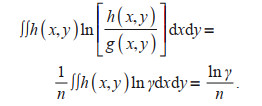
Theorem 1: Let the continuous random variables X and Y reach the maximum information entropy Hg when the joint probability density function is g(x, y). Another joint probability density function of random variables X and Y under the same constraint is h(x, y) with information entropy Hh. Then the information entropy variance satisfies the following equation:
 (3)
(3)where n is the number of samples of the continuous random variable and γ is the ratio of the likelihood function of g(x, y) to h(x, y).
Proof 1: It is known from the reference (Jiang and Qian, 1992) that
 (4)
(4)Thus the information entropy variation can be:
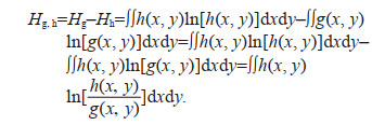 (5)
(5)The ratio of the likelihood function of h(x, y) to g (x, y) is
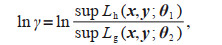 (6)
(6)where L(x, y; θi) is the likelihood function of the corresponding distribution, x with y is the measured data vector, and θi is the parameter vector.
Taking log on both sides of Eq.6, when n→ ∞ it yields
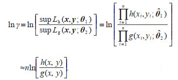 (7)
(7)Multiplying both sides of Eq.7 by h(x, y) and integration gives
 (8)
(8)Substitute Eq.8 to Eq.5 to obtain Eq.3, and Theorem 1 is proved.
When n→∞ the parameter value obtained by the maximum likelihood estimation is the parameter value of the true distribution, and thus the likelihood function values 

Corollary 1: The uncertainty due to the sample size can be calculated according to the following equation:
 (9)
(9)where n is the number of samples and Δ H1 is the change in model information entropy due to the increase in sample numbers.
Theorem 2: If the joint probability density function of continuous random variables X and Y is f(x, y) and their joint information entropy is H(x, y). The mathematical expectation and standard deviation of X are μx and σx, respectively. The mathematical expectation and standard deviation of Y are μy and σy, respectively. X and Y are normalized to X′=(X–μx)/σx and Y′=(Y–μy)/σy. The joint probability density function of X′ and Y′ probability density function is f′ (x′, y′) and the joint information entropy is Hf′. Then the following relations are obtained:
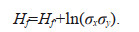 (10)
(10)Proof 2: From Eq.1, we know that
 (11)
(11)Therefore, we can have:
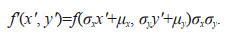 (12)
(12)Substitute Eq.12 into Eq.11 yields:
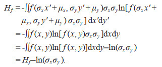 (13)
(13)Equation 10 can be obtained by rearrange the terms of Eq.13, and the Theorem 2 is proved.
From the theorem, it is clear that there is a constant difference between the joint information entropy of the multivariate model and the joint information entropy of the standardized model. This constant is the logarithmic value of the product of the standard deviations of the samples of the two variables. Since the standard deviation characterizes the dispersion of the samples, the uncertainty of the model increases with the increase of the dispersion of the data. Assuming a linear relationship between the product of the standard deviations of the samples and the joint information entropy of the multivariate model, the following corollary can be obtained.
Corollary 2: The uncertainty due to the degree of sample dispersion can be calculated according to the following equation:
 (14)
(14)where σx and σy are the standard deviations of the samples and ΔH2 is the change in information entropy due to the increase in the product of the sample standard deviations.
The choice of different multivariate models to derive the design parameters of the marine environment can introduce large uncertainties in the calculation results. Different model parameter estimation methods will in turn affect the fit of the model to the sample data. Therefore, both the model distribution and the parameter estimation method will have an impact on the uncertainty of the model. The former is defined as the uncertainty of the model itself, U3, and the latter is defined as the uncertainty caused by the parameter estimation, U4. Since the type of the distribution of the multivariate model and the parameter estimation method have certain cognitive limitations, the sum of these two uncertainties is called the epistemic uncertainty, UE. Thus there is
 (15)
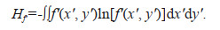
(15)where the uncertainty of the model itself can be directly obtained from the information entropy, i.e.,
 (16)
(16)where f(x, y) is the probability density function of the joint distribution.
Let the joint distribution probability density function be f (x, y; 
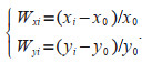 (17)
(17)Dividing the errors Wxi and Wyi into m intervals and counting the frequencies pxk and pyk occurring in the kth interval, the uncertainty due to parameter estimation can be calculated according to the following equation:
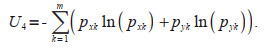 (18)
(18)The sum of the aleatory uncertainty and the epistemic uncertainty of the model is referred to as the overall uncertainty U of the model, i.e.,
 (19)
(19)Simulation data satisfying a specific multivariate model can be easily generated using Monte Carlo methods. In this paper, the Gibbs sampling method (Geman and Geman, 1984) is used. It should be noted that although algorithms such as the clustering algorithm (Swendsen and Wang, 1987) and the modified Gibbs sampling method (Liu, 1996) developed based on the original method are more computationally efficient. The focus of this paper is not on the comparison of the algorithms, but on whether simulation data can be obtained more easily. Since the Gibbs sampling method is easy to program for application in engineering, it is adopted in this paper. If the probability density function of a binary distribution model is f(x, y), the steps to generate simulated data using the Gibbs algorithm are shown as follows:
1. A random initial state (x0, y0) is given at t=0.
2. The data (x0, y1) is obtained by sampling from the conditional probability distribution fY (y|x0).
3. The data (x1, y1) is obtained by sampling from the conditional probability distribution fX(x|y1).
4. Repeat steps 2–3 to rotate the axes for sampling and obtain the data (x1, y2), (x2, y2), (x2, y3), ....
3 APPLICATIONS IN SOUTH CHINA SEA 3.1 Ocean data analysisIn this paper, we use the measured wind speed and storm surge data from 1980 to 2016 at the Shanwei observatory in the South China Sea (noted as data set D0, missing the year 2004 and 2007). The location of the station and the measured data are shown in Figs. 1–2. The red dot in Fig. 1 is the location of the station. The blue bars in the Fig. 2a–b are the measured wind speed and storm surge data (i.e., data set D0), and the red bars are the annual extreme wind speed (Vw) and annual extreme storm surge (Hs) data (noted as data set D1). Figure 2c–d shows the autocorrelation functions of Vw and Hs, from which it can be concluded that annual extreme wind speed data and annual extreme storm surge data are free from serial dependence.

|
| Fig.1 Location of the site (the red dot) Gray dotted boundary is the special adminstrative region. Map review No. GS(2019)1694. |

|
| Fig.2 Measured data and annual extreme sampling data a. measured and annual extreme wind speed (Vw) at Shanwei observatory; b. measured and annual extreme storm surge (Hs) at Shanwei observatory; c-d. autocorrelation Function (ACF) of annual extreme Vw and Hs. |
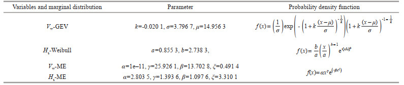
In marine engineering, the commonly used one-dimensional models for fitting extreme value data are Gumbel, Weibull, Pearson-Ⅲ, and Generalized Extreme Value distribution (GEV) models. The Maximum Entropy (ME) is a distribution model derived under the condition that the model information entropy is maximized as a constraint. This model can make the least assumptions about the model with the known information, so the ME model can minimize the influence generated by artificial choices. Since it is subject to the least conditional constraints, the ME model theoretically has the largest uncertainty compared to the other models. In this paper, the above five models are used to fit the Vw and Hs data, and the fitting results of the best models are shown in Figs. 3–6. The blue dots in Figs. 3–6 are the measured annual extreme data. The red line in Probability Plot and Quantile Plot is the position where the predicted value of the model is completely consistent with the empirical value. The better the model fitting effect is, the closer the blue point is to the red line. The solid red line in the Return Level Plot is the prediction curve of the model's return level, and the dotted red line is the 95% confidence interval of the prediction curve. The better the fitting effect of the model is, the closer the blue point is to the solid red line. The red line in the Density Plot is the probability density function curve of the model, and the blue histogram is the frequency distribution histogram of the measured data. The better the model fitting effect is, the closer the shape of the red curve is to that of the histogram. From these figures, it can be seen that the ME model can fit both Vw and Hs data well; the GEV model and the Weibull model can fit Vw data and Hs data respectively well. The parameters obtained by fitting Vw and Hs data using the above three models are shown in Table 1.

|
| Fig.3 GEV model fitting Vw The red line in Probability Plot and Quantile Plot is the position where the predicted value of the model is completely consistent with the empirical value. The solid red line in the Return Level Plot is the prediction curve of the model's return level, and the dotted red line is the 95% confidence interval of the prediction curve. The red line in the Density Plot is the probability density function curve of the model, and the blue histogram is the frequency distribution histogram of the measured data. Figs. 4-6 are similar with Fig. 3. |

|
| Fig.4 Weibull model fitting Hs |

|
| Fig.5 ME model fitting Vw |

|
| Fig.6 ME model fitting Hs |
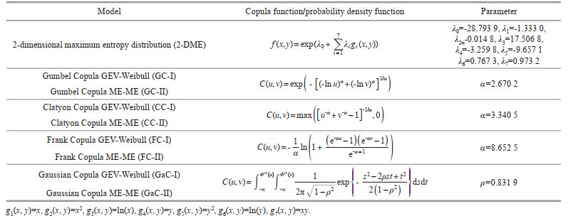
Copula functions are often used to construct multivariate probability models for better understanding of the relationships among multi variables and more reasonable probability analyzing (Grimaldi and Serinaldi, 2006). The commonly used Copula functions are Gumbel Copula, Clatyon Copula, Frank Copula, Gaussian Copula, etc. In addition to this method, the two-dimensional maximum entropy distribution (2-DME) model can be obtained under the condition that the information entropy of the model is maximum. Because the information entropy of the 2-DME model is the largest, its own uncertainty should be the largest among all binary distribution models. For further comparison and analysis, the uncertainties of the nine binary distribution models listed in Table 2 were calculated. The expressions of probability density functions of different binary distribution models and their parameters are given in Table 2.
The aleatory uncertainty of the multivariate model is directly related to the number of samples and the dispersion degree of the samples. However, due to the late development of marine environmental elements observation technology, it is difficult to obtain hundreds or thousands of years of marine environmental elements observation data in the engineering practice. Therefore, it is also difficult to calculate the aleatory uncertainty using the actual measurement data. In this paper, the Monte Carlo method mentioned in Section 2.2 is used to simulate sampling for different binary distribution models for several times, so that 10 sets of simulated Vw and Hs data are obtained (each set contains 9 models, each model concludes 1 000-Vw data and 1 000-Hs data). For the nine models mentioned in Section 3.1, the obtained simulated data are denoted as D2,2-DME, D2,GC-Ⅰ, D2,GC-Ⅱ, D2,CC-Ⅰ, D2,CC-Ⅱ, D2,FC-Ⅰ, D2,FC-Ⅱ, D2,GaC-Ⅰ, D2,GaC-Ⅱ. The details of one of the simulated data sets are shown in Fig. 7. The green dots in the Fig. 7 are simulated data, the blue dots are measured data, and the red dots are annual extreme value sampling data. From Fig. 7, it can be seen that the simulated data obtained by Monte Carlo method for each binary model can match the annual extreme value data well.

|
| Fig.7 Simulated data |
The relationship between the information entropy of the model and the number of samples is investigated using the simulation data obtained in Section 3.2. The results are shown in Fig. 8. The blue solid lines in Fig. 8 are the average values of model information entropy under 10 simulations; when sample numbers increase from 25 to 1 000, the blue dotted lines are the error line of model information entropy under different sample numbers, and the red chain-dotted lines are the regression line obtained by fitting the linearly increasing part of the blue solid lines. From Fig. 8, it can be seen that for all models, there is a tendency for the information entropy to increase first and then remain stable with the increasing number of samples. This is consistent with the results of the theoretical analysis in Section 2.1. In addition, the information entropy of the model tends to increase sharply and almost linearly with the number of samples until the model information entropy reaches the first peak. In contrast, the measured data used in this paper contain only 23 annual extreme value sampling data, and the model information entropy increases linearly with the number of samples in this case. According to this feature, Δ H1 in Eq.9 can be obtained, and the uncertainty caused by the number of samples U1 can be obtained by taking n as 23. The results are shown in Table 3. Table 3 shows that among the 9 models, the uncertainty of FC-Ⅱ model is most affected by the number of samples, while that of GaC-Ⅰ model is least affected by the number of samples.

|
| Fig.8 Variation of model information entropy with the number of samples |

From Section 2.1, it is clear that there is a close relationship between the standard deviation of the statistic reflecting the degree of sample dispersion and the information entropy of the model. For the binary model, the larger the product of the standard deviations of the samples from the two marine environmental variables, the larger the information entropy of the model. The greater the information entropy of the model represents the greater the uncertainty of the model. In other words, the more discrete the sample data is, the greater the uncertainty of the model obtained using that sample. The relationship between the dispersion of the sample and the information entropy of the model is studied using simulated data, and the results are shown in Fig. 9. The green dots in Fig. 9 are the average values of the product of the standard deviation of wind speed and storm surge samples and the average values of information entropy of the 9 models when sample numbers increase from 25 to 1 000 under 10 simulations. The red chain-dotted lines are the regression lines obtained by linear regression fitting of the green dots. The red dotted lines are the 95% confidence interval for linear regression fitting. The linear regression curve obtained by the least-square method and its 95% confidence interval encompass most of the data points as can be seen in Fig. 9. Moreover, there is a positive correlation between information entropy and the product of sample standard deviations for all nine models. This verifies the results of the theoretical analysis. The variation of the information entropy of each model due to the variation of sample dispersion ΔH2 can be obtained from Fig. 9. The standard deviations σx and σy of the measured Vw and Hs data are 4.723 3 and 0.304 4, respectively. The uncertainty U2 due to the sample dispersion can be obtained by bringing the above data into Eq.14. The calculation results are shown in Table 4, showing that among the 9 models, the uncertainty of 2-DME model is most affected by the dispersion of samples, while that of CC-Ⅰ model is least affected by the number of samples.

|
| Fig.9 Sample dispersion and model information entropy |

Since the uncertainty of the model itself can be obtained directly according to the definition of joint information entropy, and the joint information entropy can be calculated according to the probability density function of the model, there is no need to conduct simulation after the model parameters were obtained. Figure 10 shows the probability density function of each model based on the actual sampling data of annual extreme wind speed and storm surge. The 5 curves (curves with the same color are regarded as the same curve) in each subplot in Fig. 10 are the probability density function contour lines of this model. The color of these five curves becomes lighter from inside to outside, and the probability density function values they represent are 10-1, 10-2, 10-4, 10-6, and 10-8, respectively. From Fig. 10, it can be seen that the probability density contour plots of the models are very close when the same Copula function is used to construct the binary model. The calculated uncertainties of the model itself, U3, are also very close. However, when different Copula functions are used to construct the binary model, the probability density contour plots of the models are more different from each other. This indicates that the ability of the multivariate model to better describe the relationship between the marginal distributions compared to the choice of the marginal distribution is a factor that has a greater impact on the uncertainty of the model. Based on the model parameter estimation results in Tables 1–2, the uncertainty U3 of the model itself can be calculated using Eq.16, and the results are shown in Table 5. It can be seen in Table 5 that the 2-DME model has the largest U3, while the other 8 models have relatively close U3, especially when the same Copula function is used, the difference between the two models' U3 is less than 2%.

|
| Fig.10 Contour plot of probability density function for each model |

The joint return period is defined as 1/(1–F(x, y)), where F(x, y) is the cumulative distribution function of the model. The 100-year encounter joint design values (x0, y0) of each model were obtained according to the parameters listed in Tables 1–2 under the assumption that the probabilities of Vw and Hs are comparable. Ten thousands simulations were performed by Monte Carlo method, and 1 000 Vw and Hs data for different models were obtained for each simulation. The empirical distribution function is used to obtain the 100-year encounter Vw and Hs joint design values (xi, yi) for each simulation. From this, 10 000 sets of Vw and Hs joint design values were obtained. The relative error due to parameter estimation was calculated by Eq.17, splitting which evenly into 50 intervals to get the frequency and the uncertainty U4 due to parameter estimation was obtained by Eq.18. Frequencies from every interval are shown in Fig. 11. The blue histogram in Fig. 11 shows the relative error of Vw and the red histogram shows the relative error of Hs. Figure 11 shows that the relative error range of the 2-DME model is (-0.2, 0.6), and the relative error ranges of the other 8 distributions are much smaller than (-0.2, 0.6). Therefore, from Fig. 11, we can conclude that the 2-DME model has the largest uncertainty due to parameter estimation among the 9 models. As can be seen from Table 6, the uncertainty due to parameter estimation (U4) of the 2-DME model is 6.678 2, which is also significantly bigger than that of the other 8 models. It indicates that conclusion in Fig. 11 corresponds to the calculation results in Table 6 and U4 calculated by Eq.18 can correctly reflect the uncertainty caused by parameter estimation of the model.

|
| Fig.11 Relative error of prediction results of each model |

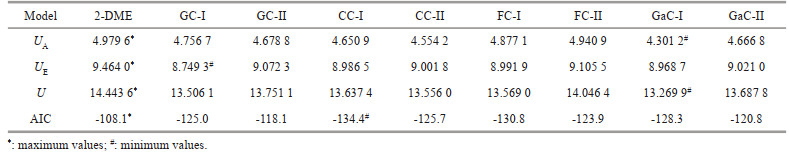
The Akaike information criterion (AIC) is based on the concept of information entropy and is often used to describe the goodness-of-fit of a model (Akaike, 2011; Xu and Guedes, 2021). This criterion assumes that the smaller the AIC value of the model the better the model fit is. The results of calculating the uncertainty and AIC values for each model are given in Table 7. From Table 7, it can be seen that the AIC information criterion indicates that 2-DME model has the worst goodness-of-fit while CC-Ⅰ model has the best goodness-of-fit. Therefore, from the perspective of goodness-of-fit, CC-Ⅰ model should be selected as the optimal model. This conclusion is consistent with the conclusion obtained from U2 and U3. However, it is different from the conclusion obtained from U1 and U4. This indicates that the commonly used test method, although it can evaluate the goodness-of-fit of the model, does not reflect the uncertainty introduced to the model due to the sample size as well as the parameter estimation. Therefore, using AIC to evaluate the goodness-of-fit of the model may result in model over-fitting problem. That is, although the model fits the sample data well, the extrapolation results are not accurate due to the large uncertainty of the model. The following conclusions can thus be drawn from the evaluation of the model from the perspective of model uncertainty. Based on the aleatory uncertainty (UA) of the model, the GaC- Ⅰ model is the best and the 2-DME model is the worst. According to the epistemic uncertainty (UE) of the model, the GC- Ⅰ model is the best and the 2-DME model is the worst. According to the principle of minimum overall uncertainty (U) of the model, GaC- Ⅰ model is the best and 2-DME model is the worst, therefore, GaC-Ⅰ model should be selected as the optimal model. It can be seen that the optimal model based on goodness-of-fit is different from that based on the principle of minimum overall uncertainty of the model. Since the length of the data used in this paper is only 23 years, it belongs to the case of small sample size. The annual extreme value data obtained based on extreme value sampling method is too short to represent the distribution characteristics of all data of marine environmental elements in nature, so we should choose the optimal model obtained by the principle of minimum overall uncertainty of the model. If the size of sample is large enough, the optimal model obtained by goodness-of-fit should be selected.
Assuming that the probabilities of Vw and Hs are comparable, the multi-year joint design values of each model are calculated under different joint return periods, and the results are shown in Fig. 12. It can be seen from the Fig. 12 that the joint design values obtained by each model have the same trend of change, whether Vw or Hs, and whether the extreme value distribution (Type-Ⅰ) or the maximum entropy distribution (Type-Ⅱ) is used as the marginal distribution. That is, the positions of the joint design value curves of each model are 2-DME, FC-Ⅰ/Ⅱ, GaC-Ⅰ/Ⅱ, GC-Ⅰ/Ⅱ, and CC-Ⅰ/Ⅱ in the order from high to low. This trend is consistent with the trend of the uncertainty of the model itself U3. And with the calculation results of 2-DME as reference, it can be seen that the joint design value curves of FC-Ⅰ, GaC-Ⅰ, GC-Ⅰ, and CC-Ⅰ models are lower than those of FC-Ⅱ, GaC-Ⅱ, GC-Ⅱ, and CC-Ⅱ models. Also, the U3 of FC-Ⅰ, GaC-Ⅰ, GC-Ⅰ, and CC-Ⅰ models in Table 5 are all smaller than the U3 of FC-Ⅱ, GaC-Ⅱ, GC-Ⅱ, and CC-Ⅱ models. Therefore, it can be considered that the larger the model's own uncertainty U3 is, the wider the range of model distribution and the larger the joint design value of the model under the same joint return period.

|
| Fig.12 Joint design values of wind speed and storm surge a–b. design values of extreme wind speed (Vw) under different joint return periods (JRP); c–d. design values of extreme storm surge (Hs) under different joint return periods (JRP). |
The uncertainty of the model for the calculation of marine environmental design parameters in the South China Sea was analyzed. The uncertainty of the model was divided into two categories according to the source of uncertainty. The first type is the aleatory uncertainty originated from samples with random nature. Both the number of samples and the dispersion of the samples have a significant effect on the aleatory uncertainty of the model. As the number of samples increases, the aleatory uncertainty of the model tends to increase linearly and then stabilizes, and tends to increase linearly as the dispersion of the samples increases. The second type is the epistemic uncertainty resulted from the model itself. Both the distribution of the model and the estimation method of the model parameters have a direct impact on the epistemic uncertainty of the model. For the South China Sea, the model with the smallest aleatory uncertainty is the GaC-Ⅰ model, but the model with the smallest epistemic uncertainty is the GC-Ⅰ model.
In the South China Sea, among the nine binary models, the 2-DME model has the highest information entropy and it is subject to the least artificial settings. Theoretically, the 2-DME model should be the model that is most consistent with the natural state. However, because it is subject to the least constraints, the 2-DME model has the largest overall uncertainty and all kinds of uncertainties. In addition, its goodness-of-fit is the worst. The GaC-Ⅰ model has the lowest overall uncertainty among the nine models, but its goodness-of-fit is in the 3rd place. The ability of the binary model to better describe the relationship between the two marginal distributions is a more influential factor on the epistemic uncertainty of the model than choosing the marginal distribution that fits samples better. The better model can be selected with reference to the overall uncertainty of the model when the models are closer in their goodness-of-fit. Doing so can ensure a better fit and avoid the situation where the model uncertainty is too high due to making too few assumptions about the model. From the analysis of the joint design values of wind speed and storm surge in the South China Sea under different models it can be concluded that the effect of the model's own uncertainty U3 on the joint design values is more obvious among the various uncertainties of the model.
The method and discussion we proposed have broad development and application prospects. First, the principle of minimum overall uncertainty of model we presented can be used for model selection when sample size is small. If the size of sample is large enough, when the optimal model based on this principle and the optimal model based on traditional methods are not the same model, how to choose the optimal model needs further study. Secondly, in addition to the uncertainty of the model U4 itself, the specific impact of other uncertainties of the model on the calculation results of marine environmental design parameters needs to be further studied. Finally, the uncertainty assessment method of multivariate model we proposed is not limited to the calculation model of marine environmental design parameters, but can also be applied to the uncertainty calculation of multidimensional probability models commonly used in finance, hydrology, and other fields.
5 DATA AVAILABILITY STATEMENTThe datasets generated during and/or analyzed during the current study are available from the corresponding author on reasonable request.
Aarnes O J, Abdalla S, Bidlot J R, et al. 2015. Marine wind and wave height trends at different ERA-interim forecast ranges. Journal of Climate, 28(2): 819-837.
DOI:10.1175/JCLI-D-14-00470.1 |
Acitas S, Aladag C H, Senoglu B. 2019. A new approach for estimating the parameters of Weibull distribution via particle swarm optimization: an application to the strengths of glass fibre data. Reliability Engineering & System Safety, 183: 116-127.
DOI:10.1016/j.ress.2018.07.024 |
Akaike H. 2011. Akaike's information criterion. In: Lovric M ed. International Encyclopedia of Statistical Science. Springer, Berlin, Heidelberg, https://doi.org/10.1007/978-3-642-04898-2.
|
Alexander C, Sarabia J M. 2012. Quantile uncertainty and value-at-risk model risk. Risk Analysis, 32(8): 1293-1308.
DOI:10.1111/J.1539-6924.2012.01824.X |
Bai X Y, Jiang H, Li C, et al. 2020. Joint probability distribution of coastal winds and waves using a log-transformed kernel density estimation and mixed copula approach. Ocean Engineering, 216: 107937.
DOI:10.1016/j.oceaneng.2020.107937 |
Blasone R S, Madsen H, Rosbjerg D. 2008. Uncertainty assessment of integrated distributed hydrological models using GLUE with Markov chain Monte Carlo sampling. Journal of Hydrology, 353(1-2): 18-32.
DOI:10.1016/J.JHYDROL.2007.12.026 |
Bruserud K, Haver S, Myrhaug D. 2018. Joint description of waves and currents applied in a simplified load case. Marine Structures, 58: 416-433.
DOI:10.1016/j.marstruc.2017.12.010 |
Chen B Y, Kou Y, Wang Y F, et al. 2021a. Analysis of storm surge characteristics based on stochastic process. IMS Mathematics, 6(2): 1177-1190.
DOI:10.3934/math.2021072 |
Chen B Y, Kou Y, Wu F, et al. 2021b. Study on evaluation standard of uncertainty of design wave height calculation model. Journal of Oceanology and Limnology, 39(4): 1188-1197.
DOI:10.1007/S00343-020-0327-8 |
Chen B Y, Kou Y, Zhao D L, et al. 2021c. Maximum entropy distribution function and uncertainty evaluation criteria. China Ocean Engineering, 35(2): 238-249.
DOI:10.1007/S13344-021-0021-4 |
Chen B Y, Zhang K Y, Wang L P, et al. 2019a. Generalized extreme value-Pareto distribution function and its applications in ocean engineering. China Ocean Engineering, 33(2): 127-136.
DOI:10.1007/S13344-019-0013-9 |
Chen W S, Mo J H, Du X, et al. 2019b. Biomimetic dynamic membrane for aquatic dye removal. Water Research, 151: 243-251.
DOI:10.1016/j.watres.2018.11.078 |
Cont R. 2006. Model uncertainty and its impact on the pricing of derivative instruments. Mathematical Finance, 16(3): 519-547.
DOI:10.1111/J.1467-9965.2006.00281.X |
de Michele C, Salvadori G. 2005. Some hydrological applications of small sample estimators of generalized Pareto and extreme value distributions. Journal of Hydrology, 301(1-4): 37-53.
DOI:10.1016/J.JHYDROL.2004.06.015 |
Silva V P R, Filho A F B, Almeida R S R, et al. 2016. Shannon information entropy for assessing space-time variability of rainfall and streamflow in semiarid region. Science of the Total Environment, 544: 330-338.
DOI:10.1016/j.scitotenv.2015.11.082 |
Derwent R G. 2020. Monte Carlo analyses of the uncertainties in the predictions from global tropospheric ozone models: tropospheric burdens and seasonal cycles. Atmospheric Environment, 231: 117545.
DOI:10.1016/j.atmosenv.2020.117545 |
Geman S, Geman D. 1984. Stochastic relaxation, Gibbs distributions, and the Bayesian restoration of images. IEEE Transactions on Pattern Analysis and Machine Intelligence, PAMI-6(6): 721-741.
DOI:10.1109/TPAMI.1984.4767596 |
Grimaldi S, Serinaldi F. 2006. Asymmetric copula in multivariate flood frequency analysis. Advances in Water Resources, 29(8): 1155-1167.
DOI:10.1016/j.advwatres.2005.09.005 |
Guachamin-Acero W, Li L. 2018. Methodology for assessment of operational limits including uncertainties in wave spectral energy distribution for safe execution of marine operations. Ocean Engineering, 165: 184-193.
DOI:10.1016/j.oceaneng.2018.07.032 |
Guan Q S, Peng W. 2015. Parameter estimation for geometric-Gumbel compound extreme-value distribution based on the pi-th quantiles of samples. In: Proceedings of 2015 Conference on Informatization in Education, Management and Business. Atlantis Press, Guangzhou, p. 60-64, https://doi.org/10.2991/iemb-15.2015.12.
|
Hora S C. 1996. Aleatory and epistemic uncertainty in probability elicitation with an example from hazardous waste management. Reliability Engineering & System Safety, 54(2-3): 217-223.
DOI:10.1016/S0951-8320(96)00077-4 |
Huang W N, Dong S. 2020. Joint distribution of individual wave heights and periods in mixed sea states using finite mixture models. Coastal Engineering, 161: 103773.
DOI:10.1016/j.coastaleng.2020.103773 |
Jiang D, Qian Y M. 1992. Information Theory and Coding. University of Science and Technology of China, Hefei, China. p. 353-399. (in Chinese)
|
Kurian V J, Nizamani Z, Liew M S. 2012. Statistical modelling of environmental load uncertainty for jacket platforms in Malaysia. In: Proceedings of 2012 IEEE Colloquium on Humanities, Science and Engineering. IEEE, Kota Kinabalu, Malaysia. p. 74-79, https://doi.org/10.1109/chuser.2012.6504284.
|
Lei F H, Xie B T, Wang J Q. 2012. Uncertainty analysis of marine environment elements calculation. The Ocean Engineering, 30(4): 109-117.
(in Chinese with English abstract) DOI:10.16483/j.issn.1005-9865.2012.04.019 |
Li Y X, Liu G L. 2020. Risk analysis of marine environmental elements based on Kendall return period. Journal of Marine Science and Engineering, 8(6): 393.
DOI:10.3390/JMSE8060393 |
Liu D F, Dong S, Wang C. 1996. Uncertainty and sensitivity analysis of reliability for marine structures. In: Proceedings of the 6th International Offshore and Polar Engineering Conference. ISOPE, Los Angeles, USA. p. 380-386.
|
Liu D F, Wang L P, Pang L. 2006. Theory of multivariate compound extreme value distribution and its application to extreme sea state prediction. Chinese Science Bulletin, 51(23): 2926-2930.
DOI:10.1007/S11434-006-2186-X |
Liu G L, Chen B Y, Gao Z K, et al. 2019a. Calculation of joint return period for connected edge data. Water, 11(2): 300.
DOI:10.3390/w11020300 |
Liu G L, Chen B Y, Jiang S, et al. 2019b. Double entropy joint distribution function and its application in calculation of design wave height. Entropy, 21(1): 64.
DOI:10.3390/E21010064 |
Liu G L, Cui K, Jiang S, et al. 2021. A new empirical distribution for the design wave heights under the impact of typhoons. Applied Ocean Research, 111: 102679.
DOI:10.1016/j.apor.2021.102679 |
Liu G L, Yu Y H, Kou Y, et al. 2020. Joint probability analysis of marine environmental elements. Ocean Engineering, 215: 107879.
DOI:10.1016/j.oceaneng.2020.107879 |
Liu J S. 1996. Peskun's theorem and a modified discrete-state Gibbs sampler. Biometrika, 83(3): 681-682.
DOI:10.1093/biomet/83.3.681 |
Ma C H, Huang Q, Guo A J. 2019. Characteristic analysis and uncertainty assessment of joint distribution of flow and sand in Jinghe River basin. Journal of Hydraulic Engineering, 50(2): 273-282.
(in Chinese with English abstract) DOI:10.13243/j.cnki.slxb.20180669 |
Ma P F, Zhang Y. 2022. Modeling asymmetrically dependent multivariate ocean data using truncated copulas. Ocean Engineering, 244: 110226.
DOI:10.1016/j.oceaneng.2021.110226 |
Meng S J, Meng X H, Fan W H, et al. 2020. The role of transparent exopolymer particles (TEP) in membrane fouling: a critical review. Water Research, 181: 115930.
DOI:10.1016/j.watres.2020.115930 |
Negnevitsky M, Terry J, Nguyen T. 2014. Using information entropy to quantify uncertainty in distribution networks. In: Proceedings of 2014 Australasian Universities Power Engineering Conference. IEEE, Perth, Australia. p. 1-6, https://doi.org/10.1109/AUPEC.2014.6966487.
|
Nugues P M. 2014. Topics in information theory and machine learning. In: Nugues P M ed. Language Processing with Perl and Prolog. Springer, Berlin, Heidelberg. p. 87-121, https://doi.org/10.1007/978-3-642-41464-0_4.
|
Panchang V, Zhao L Z, Demirbilek Z. 1998. Estimation of extreme wave heights using GEOSAT measurements. Ocean Engineering, 26(3): 205-225.
DOI:10.1016/S0029-8018(97)10026-9 |
Petrov V, Guedes Soares C, Gotovac H. 2013. Prediction of extreme significant wave heights using maximum entropy. Coastal Engineering, 74: 1-10.
DOI:10.1016/j.coastaleng.2012.11.009 |
Shannon C E. 1948. A mathematical theory of communication. The Bell System Technical Journal, 27(3): 379-423.
DOI:10.1002/j.1538-7305.1948.tb01338.x |
Silva-González F, Heredia-Zavoni E, Inda-Sarmiento G. 2017. Square error method for threshold estimation in extreme value analysis of wave heights. Ocean Engineering, 137: 138-150.
DOI:10.1016/j.oceaneng.2017.03.028 |
Swendsen R H, Wang J S. 1987. Nonuniversal critical dynamics in Monte Carlo simulations. Physical Review Letters, 58(2): 86-88.
DOI:10.1103/physrevlett.58.86 |
Tapiero O J. 2013. The relationship between risk and incomplete states uncertainty: a Tsallis entropy perspective. Algorithmic Finance, 2(2): 141-150.
DOI:10.3233/AF-13022 |
Vanem E. 2016. Joint statistical models for significant wave height and wave period in a changing climate. Marine Structures, 49: 180-205.
DOI:10.1016/j.marstruc.2016.06.001 |
Wang L P, Chen B Y, Chen C, et al. 2016. Application of linear mean-square estimation in ocean engineering. China Ocean Engineering, 30(1): 149-160.
DOI:10.1007/S13344-016-0007-9 |
Wist H T, Myrhaug D, Rue H. 2004. Statistical properties of successive wave heights and successive wave periods. Applied Ocean Research, 26(3-4): 114-136.
DOI:10.1016/j.apor.2005.01.002 |
Wu M N, Gao Z. 2021. Methodology for developing a response-based correction factor (alpha-factor) for allowable sea state assessment of marine operations considering weather forecast uncertainty. Marine Structures, 79: 103050.
DOI:10.1016/J.MARSTRUC.2021.103050 |
Wu M N, Stefanakos C, Gao Z, et al. 2019. Prediction of short-term wind and wave conditions for marine operations using a multi-step-ahead decomposition-ANFIS model and quantification of its uncertainty. Ocean Engineering, 188: 106300.
DOI:10.1016/j.oceaneng.2019.106300 |
Xu S, Guedes Soares C. 2021. Evaluation of spectral methods for long term fatigue damage analysis of synthetic fibre mooring ropes based on experimental data. Ocean Engineering, 226: 108842.
DOI:10.1016/J.OCEANENG.2021.108842 |
Zachary S, Feld G, Ward G, et al. 1998. Multivariate extrapolation in the offshore environment. Applied Ocean Research, 20(5): 273-295.
DOI:10.1016/S0141-1187(98)00027-3 |
Zhai J J, Yin Q L, Dong S. 2017. Metocean design parameter estimation for fixed platform based on copula functions. Journal of Ocean University of China, 16(4): 635-648.
DOI:10.1007/S11802-017-3327-3 |
Zhang H D, Guedes Soares C. 2016. Modified joint distribution of wave heights and periods. China Ocean Engineering, 30(3): 359-374.
DOI:10.1007/S13344-016-0024-8 |
Zhang H D, Liao X M, Shi H D, et al. 2022. Effect of initial condition uncertainty on the profile of maximum wave. Marine Structures, 82: 103127.
DOI:10.1016/j.marstruc.2021.103127 |
Zhang S, Solari G, Yang Q S, et al. 2018. Extreme wind speed distribution in a mixed wind climate. Journal of Wind Engineering and Industrial Aerodynamics, 176: 239-253.
DOI:10.1016/J.JWEIA.2018.03.019 |
Zhang W X, Grimi N, Jaffrin M Y, et al. 2015a. Leaf protein concentration of alfalfa juice by membrane technology. Journal of Membrane Science, 489: 183-193.
DOI:10.1016/j.memsci.2015.03.092 |
Zhang W X, Jiang F. 2019. Membrane fouling in aerobic granular sludge (AGS) -membrane bioreactor (MBR): effect of AGS size. Water Research, 157: 445-453.
DOI:10.1016/j.watres.2018.07.069 |
Zhang W X, Liang W Z, Zhang Z E, et al. 2021. Aerobic Granular Sludge (AGS) scouring to mitigate membrane fouling: performance, hydrodynamic mechanism and contribution quantification model. Water Research, 188: 116518.
DOI:10.1016/j.watres.2020.116518 |
Zhang Y. 2015. On the climatic uncertainty to the environment extremes: a Singapore case and statistical approach. Polish Journal of Environmental Studies, 24(3): 1413-1422.
DOI:10.15244/pjoes/31718 |
Zhang Y, Cao Y Y. 2015. A fuzzy quantification approach of uncertainties in an extreme wave height modeling. Acta Oceanologica Sinica, 34(3): 90-98.
DOI:10.1007/s13131-015-0636-5 |
Zhang Y, Cao Y Y, Dai J. 2015b. Quantification of statistical uncertainties in performing the peak over threshold method. Journal of Marine Science and Technology, 23(5): 15.
DOI:10.6119/JMST-015-0604-1 |
Zhang Y, Lee Lam J S. 2014. Non-conventional modeling of extreme significant wave height through random sets. Acta Oceanologica Sinica, 33(7): 125-130.
DOI:10.1007/s13131-014-0508-4 |
Zhu Z Z, Chen Z, Luo X, et al. 2020. Gravity-Driven Biomimetic Membrane (GDBM): an ecological water treatment technology for water purification in the open natural water system. Chemical Engineering Journal, 399: 125650.
DOI:10.1016/j.cej.2020.125650 |