 2023, Vol. 41
Institute of Oceanology, Chinese Academy of Sciences
Article Information
- HOU Guangchao, ZHAI Jingsheng, SHAO Qi, ZHAO Yanling, LI Wei, HAN Guijun, LIANG Kangzhuang
- Sound speed profiles in high spatiotemporal resolution using multigrid three-dimensional variational method: a coastal experiment off northern Shandong Peninsula
- Journal of Oceanology and Limnology, 41(1): 57-71
- http://dx.doi.org/10.1007/s00343-022-1295-y
Article History
- Received Sep. 8, 2021
- accepted in principle Nov. 8, 2021
- accepted for publication Jan. 14, 2022


2 Tianjin Key Laboratory for Oceanic Meteorology, Tianjin 300074, China;
3 The PLA 31010 Units, Beijing 100081, China
The undersea acoustic activities are highly correlated with seawater sound speed profiles (SSPs) in coastal areas, especially in the field of hydrographic surveys (Church, 2020). It is well known that the measurement accuracy of modern sonar sounding equipment (Multi-Beam Echo-Sounder, MBES) based on acoustic time-of-arrival ranging is greatly degraded due to the lack of sufficient high-precision spatiotemporal resolution SSPs. Besides, SSPs are complex and changeable in coastal areas. However, there are few studies on the construction method of high spatiotemporal resolution SSPs due to the complex environment of the coastal areas and observational deficiency over there. Therefore, it is extremely crucial to obtain high-resolution SSPs based on available observations in coastal areas, including sound velocity observations, temperature-salinity observations.
In general, Sound Velocity Profiler (SVP) (Didier et al., 2019) is used to directly obtain SSPs in the traditional SSPs measurement method. In addition, the other way is to measure salinity, temperature and static pressure of the immediate ocean water column through Conductivity Temperature Depth (CTD) profiler and then obtain the SSPs by the sound velocity empirical formula (Jamshidi and Abu Bakar, 2011). On the one hand, it is impossible to obtain high spatiotemporal resolution SSPs by these traditional stop-and-start measurement methods, which cost plenty of time to do the survey. On the other hand, these traditional SSPs observation methods cannot meet the high precision requirements of modern hydrographic surveying since these traditional methods assume that the time scales of sound velocity changes are much longer than the standard in-situ sampling period of SSPs. Since the late 1990s, the underway sound velocity profiler (known as moving vessel profiler, MVP) has been used to obtain high spatiotemporal resolution SSPs to provide hydrographers with an unprecedented ability to sample the sound velocity through which they sample the seafloor (Furlong et al., 1997). However, the capital costs and ongoing maintenance costs of MVP are both much higher than traditional SSPs observation instruments due to the increasing sophistication in deployment hardware and control components. In addition, the vast majority of hydrographic survey vessels do not have underway SSPs capability.
Recently, many studies have shown that the subsurface temperature field can be inferred from sea surface height anomaly (SSHa) and sea surface temperature (SST) by the physical relation based on the fact that the heat expansion and contraction of seawater (Fox et al., 2002; Wang et al., 2013). In the deep ocean area, subsurface salinity can be calculated from the above subsurface temperature (there exists a stable relationship between them (Mamayev, 2010) since the deep ocean areas are dominated by the first baroclinic modes (Wunsch, 1997; Shinoda, 2012)), and then the high spatiotemporal resolution SSPs can be further calculated through the empirical formula of undersea sound velocity. Chen et al. (2020) reconstruct the SSPs directly from SSHa and SST using a self-organizing map method (SOM), which is more suitable for nonlinear dynamics in the deep ocean areas. However, the applicability of the method in the shallow sea regions is still very poor. First of all, this is due to the very poor quality of SSHa in the nearshore shallow coastal areas, which makes it impossible to obtain a high-quality subsurface temperature field. In addition, the shallow sea regions are dominated by the barotropic signal. The above two factors make it impossible to obtain the subsurface salinity field from the subsurface temperature field in coastal sea areas.
Ocean data assimilation schemes have been substantially developed since the mid-1980s through which the observation and background information in space-time dimension, as well as physics constraints, have been fully used (Bocquet et al., 2010; Edwards et al., 2015; Bannister, 2017; Carrassi et al., 2018), including the variational data assimilation (3DVar (Fu et al., 2012; Fu, 2013), 4DVar (Powell et al., 2008a, b; Carrier et al., 2014; Ngodock and Carrier, 2014)), the ensemble data assimilation (ensemble Kalman filter (EnKF) (Evensen, 2003; Keppenne et al., 2005; Shu et al., 2011; Houtekamer and Zhang, 2016)), and the ensemble-variational (EnVar) (Liu and Xiao, 2013; Desroziers et al., 2014; Liu and Xue, 2016; Liang et al., 2021). The 3DVar is an important tool for numerical forecast and reanalysis of the ocean. Compared with other ocean data assimilation methods, one of 3DVar's advantages is that some constraints terms can be introduced. The traditional 3DVar method usually uses the correlation scale method (Derber and Rosati, 1989) and the recursive filtering method (Hayden and James Purser, 1995) to construct the background field error covariance matrix (B). Regardless of whether the correlation scale method or the recursive filtering method is used to construct B, only the information of a specific wavelength can be extracted due to the static characteristics of the traditional 3DVar method, and the short-wave information cannot be extracted well if the long-wave information is not extracted well.
To quickly and sequentially minimize the longwave and shortwave errors, a multigrid 3DVar approach (in this paper, we call it MG3DVar) has been proposed by Xie et al. (2005). By using the MG3DVar, Li et al. (2008) assimilate the sea surface temperature (SST) and temperature profile observations to predict the China Seas' temperature, and this scheme has higher forecast accuracy and lower root-mean-square errors than that of the traditional 3DVar.
In this study, we proposed a method, the space-time multigrid 3DVar data assimilation scheme with temperature-salinity constraint terms (STC-MG3DVar), for constructing high spatiotemporal resolution SSPs in coastal areas using sound velocity and temperature-salinity observations based on the MG3DVar method described above. In this method, sound velocity is defined as the control variable of the cost function. First, the spatiotemporal correlation and multiscale information of sound velocity observations can be effectively considered in the STC-MG3DVar method. Besides, it is well known that sound velocity is highly correlated with the ocean's temperature-salinity fields, and high-precision temperature-salinity observations may effectively reflect the variation of the sound velocity field in turn. Therefore, we introduce the Chen-Millero sound velocity empirical formula as a weak constraint into the cost function of the STC-MG3DVar, which can improve the SSPs' accuracy through the physical relationship between sound velocity and temperature-salinity. To validate the accuracy of the STC-MG3DVar method for constructing high spatial and temporal resolution SSPs, we obtained 27 sets of CTD (temperature profile and salinity profile) and SSPs observation profiles in the northern coastal area of the Shandong Peninsula.
The remainder of the paper is organized as follows: Section 2 describes the study area and data used in this study, and the detailed methodology is also presented in this section. In Section 3, we present the setup of experiments and the performance evaluation criteria. The results and discussions are illustrated and discussed in Section 4. Section 5 is our conclusion of the study.
2 DATA AND METHOD 2.1 SVP and CTD observation profile dataIn this study, we measured SSPs observations by the Valeport Sound-Velocity-Profiler (called "MiniSVP", Valeport Ltd., United Kingdom) instrument and CTD profile observations (including temperature profile (TP) and salinity profile (SP) observations) by the Valeport Conductivity-Temperature-Depth profiler (called "MiniCTD") in the northern coastal area of the Shandong Peninsula. The experimental area includes the North Yellow Sea of China in an area of 37.575°N–37.605°N, 122.06°E–122.12°E, as shown in Fig. 1. The depth of this experimental area approximately ranges from 25 to 70 m. The approximate locations of these field observation stations are shown in Fig. 1. The "MiniSVP" and "MiniCTD" instruments were deployed together during this ocean survey on June 8, 2019, and SSPs observations and CTD observations are observed at each observation station. As shown in Fig. 1, we measured Nos. 1–27 observation station, and the observations were sampled at 1 Hz. A set of TP, SP, and SSPs were observed at each observation station during each deployment. Only one set of observations per observation station, and each station has both sound velocity observations and temperature-salinity observations. In this study, we used the bathymetric data measured by the Multibeam Echosounder (called "R2SONIC 2024", R2Sonic LLC, USA) and the Singlebeam Echosounder (called "Haiying Y1200", Wuxi Haiying-Cal Tec Marine Technology Co. Ltd., China) as the boundary of the seabed topography (as shown in Fig. 1).

|
| Fig.1 The study area and the space distribution of field observation stations The red five-pointed star indicates the observation stations used as validation data in the experiment, while the black solid circle indicates the observation stations used as experimental data. |
SSPs, TP, and SP observations are presented in Fig. 2. Different colors are just used to denote profile observations at different stations without any other meanings. The changing trends of sound velocity are consistent with those of temperature and salinity, especially a high correlation with temperature, which follows the physical properties of oceanic sound velocity (Fig. 2). Quality control of the SVP and CTD observation profile data includes automatic quality control, gross validity checks, temporal consistency checks, and spatial checks. Since the main content of this paper is to investigate the feasibility of the STC-MG3DVar method in the construction of high-precision spatiotemporal resolution SSPs, the detailed quality control of observational data will not be described here. Besides, we interpolated the SSPs, TP, and SP to 0.2-m vertical resolution using the Akima interpolation algorithm.

|
| Fig.2 Profile observations in the northern coastal area of the Shandong Peninsula a. sound velocity profile observations; b. temperature profile observations; c. salinity profile observations. |
To extract the multi-scale information of ocean observations sequentially, Xie et al. (2005) proposed a multigrid 3DVar (MG3DVar) method which can minimize the cost function on a coarse grid to obtain long-wave information, and on a relative fine grid to extract long- and short-wavelength information from the observations in turn. The basic idea of the multigrid 3DVar implementation can be found in (Xie et al., 2005; Li et al., 2008, 2010, 2013), and it is briefly reviewed here. Generally, the cost function of MG3DVar consists of two parts: background field item Jb and observation field item Jo. The cost function in the incremental form of the MG3DVar for the nth level grid takes the following form:
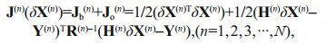 (1)
(1)where δX is the analysis increment vector, H is a simple bilinear interpolation operator from the gird to the observation location, R is the observational error covariance matrix, Y denotes the observational innovation vector, T and -1 represent the transpose matric and inverse matric, respectively; the N is the final level, which depends on the observations. Y(1)=Yobs–H(1)Xb is the difference between the observations and the interpolated background at the observation locations in the first level grid, and in the other grid levels it is defined as:
 (2)
(2)The final analysis value Xa is equal to the sum of the analysis value increment δX for all grids level and the background value Xb:
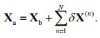 (3)
(3)In this study, the cost function of STC-MG3DVar is similar to Eq.1 and the control variable of the cost function is sound velocity increment δXSV(n). The distribution of the SVP and CTD observations is relatively homogeneous and extremely accurate, that is, complete reliance on the observation field and exclusion of the background field, so the cost function of STC-MG3DVar omits the background term Jb and the spatial extension is then represented by the grid spacing. Besides, the smooth term of sound velocity observations, at the same time, is introduced into the cost function of STC-MG3DVar to reduce the bilinear interpolation truncation error effect (Li et al., 2010) and the smoothing penalty term itself can damp small scale noise and make solution unique with enough but still sparse observations. Li et al. (2013) discussed the meaning of the smoothing term in detail. Therefore, the incremental form of the cost function of STC-3DVar for the nth level gird is simplified to:
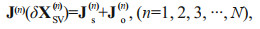 (4)
(4)where s the incremental form of control variables for the nth level gird, and in this study, N is equal to 2; the subscript s denotes the smooth term (penalty term) and o represents the SVP sensor observation data term:
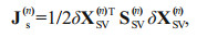 (5)
(5) (6)
(6)where the smooth matrix SSV(n) in the smooth term is derived from the spatial integral of the square of Laplacian of control variables δXSV(n) at the nth level grid points.
To obtain a more reasonable and accurate analysis of the sound velocity, the Chen-Millero sound velocity empirical formula, whose coefficients are given in Chen and Millero (1977), is incorporated into the cost function of STC-MG3DVar as a weak constraint condition. Therefore, the final cost function of STC-MG3DVar is expressed as follows:
 (7)
(7)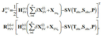 (8)
(8)where w denotes the weak constrain term; XSVb represents the background value of the seawater sound velocity, and in this study, XSVb is equal to the average of the sound velocity at each water layer; the matrix RPSVn-1 is an error covariance matrix for the empirical formula for the sound velocity of seawater; the function SV(Tobs, Sobs, P) denotes the Chen-Millero sound speed equation, Tobs, Sobs, and P are the observation values of temperature, salinity, and pressure corresponding to the sound velocity of each water layer, respectively.
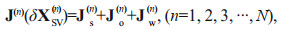
In STC-MG3DVar, the δXSV(n) ("analysis") is obtained by minimizing the cost function (Eq.7), δXSV(n)=arg min J(n)(δXSV(n)). The gradient function of the cost function is expressed:
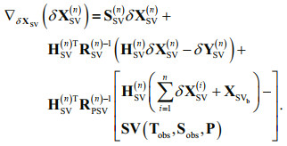 (9)
(9)Finally, the sound velocity analysis value is expressed as follow:
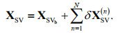 (10)
(10)To verify the accuracy of the assimilation results of different assimilation algorithms, independent sample experiments are conducted. We selected the SSPs observation data of No. 11 and No. 24 as the verification data and other remaining data as the assimilation input data. Observation data (including SSPs, TP, and SP data) from No. 11 and No. 24 observation stations (the red Pentastar as shown in Fig. 1) are only used to verify the accuracy of the assimilation results, not as input data for the assimilation experiment. The remaining observation data (the black solid circle as shown in Fig. 1) are used as input data for these assimilation experiments.
We designed six comparison experiments, and the detailed parameter settings of these six groups of comparison experiments are shown in Table 1. In all experiments, the time resolution is half an hour, the horizontal resolution is 0.002°×0.002°, and the vertical resolution is 1 m. The horizontal range of these experiments is within 37.575°N–37.605°N, 122.06°E–122.12°E. In EXP1-3, the SSPs of the No. 11 station is used as reference profile observations to verify the accuracy of SSPs constructed by different assimilation schemes, and the SSPs of the No. 24 station is used as reference profile observations in EXP4-6. In EXP1 & 2, to align the time of constructed SSPs with that of No. 11, the time range of EXP1 & 2 is set to be from 7:22:55 (UTC+08) to 11:22:55 (UTC+08), and the time resolution was half an hour (the observation time of No. 11 is 08:52:55). Similarly, the time range of EXP4 & 5 is from 07:03:23 (UTC+08) to 11:33:23 (UTC+08), and the time resolution is also half an hour (the observation time of No. 24 is 10:33:23). In addition, we set the grid points (the horizontal coordinates of the constructed SSPs) exactly at the spatial location of the independent sample observation station (the horizontal coordinates of No. 11 and No. 24).
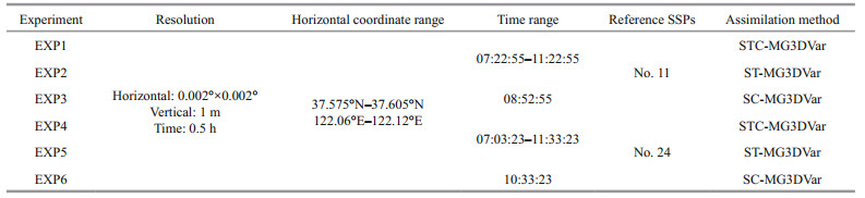
First, to investigate whether the weak constraint term can optimize sound velocity through the physical relationship between sound velocity and temperature-salinity simultaneously to obtain more reasonable and accurate SSPs, we set up EXP1 & 2 for comparison. The EXP1 uses the STC-MG3DVar to construct SSPs, and the EXP2 uses the space-time multigrid 3DVar method without the temperature-salinity constraint term (referred to as the ST-MG3DVar) to construct SSPs. Second, in the EXP3, the spatial multigrid 3DVar method with weak constraint term (referred to as the SC-MG3DVar) is used to construct SSPs, which considers that all sound velocity observations are at the same time. Third, to verify whether high-precision SSPs can be obtained at the edge of the study area, where there are few available sound velocity and thermohaline observation data within the space-time dimension radius of assimilation, the same experiments are carried out at EXP4-6.
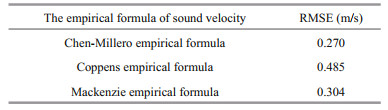
In addition, it is also the key to selecting the optimal empirical formula of sound velocity, which is most suitable for the calculation of sound velocity in our study sea areas since different sound velocity empirical formulas are strongly dependent on the respective application conditions. The most likely error sources of the sound velocity empirical formula mainly come from the different application ranges of the formula in different ocean areas. In this study, compared with the Coppens empirical formula and the Mackenzie empirical formula, the Chen-Millero sound velocity empirical formula is more suitable for the sea area of this study. The statistical errors of the three classic sound velocity empirical formulas are shown in Table 2.
The SSPs constructed by different assimilation methods (as described in Table 1) were compared with the observed SSPs to determine the accuracy of the proposed STC-MG3DVar method. In this study, we use the root-mean-square error (RMSE), the Pearson correlation coefficient (R), maximum absolute error and minimum absolute error as evaluation metrics. The RMSE can reflect the closeness of two SSPs, and the R represents the similarity between the observed SSPs and the constructed SSPs. The maximum absolute error represents the limit error of different methods and the smallest error indicates the stability of the different methods. The smaller the RMSE, the higher the accuracy of the algorithm. The closer the R is to 1, the better the results are. The smaller the maximum error and minimum error, the more stable the algorithm. If the minimum error can be small enough, it means that the SSPs constructed through our algorithm, STC-MG3DVar, is sufficiently stable. These formulas are expressed as follows:
 (11)
(11) (12)
(12) (13)
(13)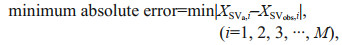 (14)
(14)where M is the number of sound velocity data in each SSP, XSVa, i is the ith value of the assimilated sound velocity, XSVobs, i is the ith sound velocity observation, XSVa is the average of all assimilation sound velocity values, and XSVobs is the average of all sound velocity observations.
4 RESULT AND DISCUSSIONBased on the experimental setup in Section 3.1, the SSPs constructed by different assimilation methods (STC-MG3DVar, ST-MG3DVar, and SC-MG3DVar) is a gridded field that changes over time, and its time resolution is half an hour, the horizontal resolution is 0.002°×0.002°, and the vertical resolution is 1 m in this study. In EXP1 & 2, a total of nine constructed SSPs are obtained at the location of the No. 11 station from 7:22:55 to 11:22:55. Similarly, in EXP4 & 5, the total number of constructed SSPs at the location of No. 24 station from 07:03:23 to 11:33:23 is 10.In EXP3 & 6, only one SSP is constructed at the location of the Nos. 11 & 24 station, since the SC-MG3DVar believes that all SSPs observations are at the same time. Table 3 presents the RMSE and R for all experiments.
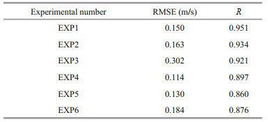
Figure 3 shows the RMSE and the R between the observed SSPs of No. 11 and these SSPs constructed by the STC-MG3DVar (EXP1) and ST-MG3DVar (EXP2). The RMSE of the STC-MG3DVar-constructed SSPs is minimal at 08:52:55 (the observation time of No. 11) with an RMSE of 0.150 m/s (Fig. 3a). Similarly, the R at this moment is a maximum value of 0.951 (Fig. 3b). The SSPs constructed by ST-MG3DVar in EXP2 has the smallest RMSE at 8:52:55 with an RMSE of 0.163 m/s (Fig. 3a). Meanwhile, the R is the maximum value at this moment with a value of 0.934 (Fig. 3b). The RMSE of STC-MG3DVar-constructed SSPs is slightly smaller than that of ST-MG3DVar-constructed SSPs at all times, and the R of the former' SSPs is greater than the latter's SSPs at all times (Fig. 3).

|
| Fig.3 The RMSE (a) and R (b) between the observed SSPs and the SSPs constructed by STC-MG3DVar (blue solid line) and ST-MG3DVar (orange dotted line) in EXP1 & 2 |
The RMSE and the R between the observed SSPs of No. 24 and these SSPs constructed by the STC-MG3DVar (EXP4) and ST-MG3DVar (EXP5) are shown in Fig. 4. The STC-MG3DVa-constructed SSP has the smallest RMSE of 0.114 m/s at 10:33:23 (the observation time of No. 24) (Fig. 4a). Meanwhile, the R is the maximum with a value of 0.897 (Fig. 4b). Clearly, the RMSE of the SSPs constructed by ST-MG3DVar is a minimum value at 10:33:23 and the RMSE is 0.130 m/s (Fig. 4a). Similarly, the R at this moment is the maximum value of 0.860 (Fig. 4b). Similarly, the RMSE of STC-MG3DVar-constructed SSPs is slightly smaller than that of ST-MG3DVar-constructed SSPs at all times, and the R of the former's SSPs is greater than the latter's SSPs at all times (Fig. 4).

|
| Fig.4 The RMSE (a) and R (b) between the observed SSPs and the SSPs constructed by STC-MG3DVar (blue solid line) and ST-MG3DVar (orange dotted line) in EXP4 & 5 |
Combining the results shown in Figs. 3–4 and Table 3, it can be seen that the STC-MG3DVar method effectively improves the accuracy of constructed SSPs, which has smaller RMSE and larger R compared with the ST-MG3DVar. The results in Table 3 show that the RMSE of the STC-MG3DVar-constructed SSPs in EXP1 (EXP4) was 7.98% (12.31%) lower than that of ST-MG3DVar in EXP2 (EXP5) at observation time (08:52:55). In the STC-MG3DVar method, the novel opportunity of assimilating temperature-salinity observations is to provide positive constraints to sound velocity, which introduces new observation information closely linked to sound velocity changes. The temperature-salinity weak constraint term can optimize the sound velocity by the physical relationship between the sound velocity and the temperature-salinity to obtain more reasonable and accurate SSPs.
In addition, the STC-MG3DVar-constructed SSPs before 9:03:23 shows a negative correlation with the observed SSPs in EXP4 (Fig. 4b). In this study, we just observed from No. 1 to No. 27 stations in sequence (Fig. 1) similar to the way of underway sailing. In other words, there is only one set of observation data at each observing station (sound velocity observations, temperature and salinity observations). As is known to all, due to the fatal shortcoming of traditional SSPs observation methods, the sound velocity observation data are very sparse in time and space. This is the fundamental reason why we proposed this algorithm in this study. Our algorithm, STC-MG3DVar, can use discrete SSPs observation data to construct high-precision spatiotemporal resolution SSPs. In EXP4, we set the time range (07:03:23–11:33:23) to approximately the time range of No. 1 and No. 27 observation station and the horizontal range is also within the space range of these observation stations. In the time dimension, it is equivalent to extrapolating in the time dimension before 9:03:20, so there will be a negative correlation coefficient. As time progressed, observation data began to participate in the assimilation of the sound velocity at the grid of the No. 24 observation station, so the correlation coefficient changes from negative to positive with time (as shown in Figs. 4–5). The sound velocity and thermohaline observations are roughly evenly distributed in the spatial dimension and cover the survey area in this study, but on the one hand, the observation data in the spatial dimension is still too few at the edge of the study area; on the other hand, the distribution of sound velocity and temperature and salinity observations in the time dimension is also extremely small. The above reasons cause the low accuracy of constructed SSPs at the edge of the study area. Due to insufficient sound velocity observation data, the accuracy of the constructed SSPs is not high enough in the marginal area of the study area. As we all know, observing sound velocity and temperature-salinity has always been difficult and costly despite its profound significance in-field measurement. Thus, how to design optimal observations in the ocean has always been critical before the beginning of ocean observation studies. In future research, we will consider adopting a model-based observation design strategy (Mu, 2013; Zhang et al., 2020), which is a systematic project seeking to observe the ocean effectively and economically to collect field sound velocity observation data, to achieve control of the sound velocity assimilation in the entire research area. In addition, we will consider adding ocean numerical models to impose dynamic constraints on the assimilation process of this method in the following research to ensure the accuracy of the SSPs constructed by the proposed method.

|
| Fig.5 The observed SSPs (the blue solid line) and the SSPs constructed by STC-MG3DVar (the red dotted line) in EXP4 |
As shown in Figs. 3–4, only the constructed SSPs which is contemporaneous with the observed SSPs can have a minimum RMSE and a maximum R. In other words, only the constructed SSPs at the same time as observed SSPs can be closer to the "real" SSPs. It is well known that the sound velocity evolves not only in the space dimension but also in the time dimension. The above experimental results also prove that the evolution of sound velocity in the time dimension in the proposed method, the STC-MG3DVar, is tenable. Furthermore, as can be seen from Table 3, the RMSE of SC-MG3DVar-constructed SSPs is 0.302 m/s and 0.184 m/s in EXP3 & 6, respectively. The RMSE results in Table 3 show that the RMSE of STC-MG3DVar-constructed SSPs in EXP1 (EXP4) was 50.33% (38.04%) lower than that of ST-MG3DVar-constructed SSPs in EXP3 (EXP6). The SC-MG3DVar believes that both sound velocity observations and thermohaline observations are at the same time, that is, the SC-MG3DVar believes that sound velocity observations and thermohaline observations were only distributed in space dimension, but not in the time dimension. In EXP3 & 6, the SC-MG3DVar does not consider the variations of the sound velocity in the time dimension, it assumes that the observed sound velocity is all at the same time. Obviously, such assumptions lead to greater errors in the SC-MG3DVar method. However, the STC-MG3DVar can extract the spatiotemporal correlation of the sound velocity observations and thermohaline observations, especially the correlation information of time dimension. Based on the above analysis, a conclusion can be drawn that the STC-MG3DVar method greatly improves the construction accuracy of SSPs compared with the SC-MG3DVar method.
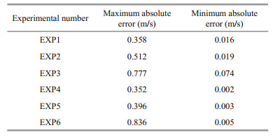
4.3 The vertical profile error of constructed SSPsThe vertical profile error of constructed SSPs is calculated at the observation time and the location of referenced SSPs in EXP1–6. In other words, only the SSP constructed at 08:52:55 is compared with the SSPs observation values of No. 11 in EXP1–3, and only the SSP constructed at 10:33:23 is compared with the SSPs observation value of No. 24 in EXP4–6. Table 4 represents the maximum absolute errors and the minimum absolute errors for all experiments.
The SSPs constructed by different assimilation methods (Fig. 6) show that the SSP constructed by STC-MG3DVar and ST-MG3DVar is much closer to the SSPs observations than the SSPs constructed by SC-MG3DVar. With the advantage of the temperature-salinity constraint term and the spatiotemporal correlation information, the STC-MG3DVar method we proposed works better than the ST-MG3DVar and the SC-MG3DVar in constructing high-precision spatiotemporal resolution SSPs.

|
| Fig.6 The observed SSPs and the constructed SSPs a. the observed SSPs of No. 11 station and the constructed SSPs at 08:52:55 in EXP1-3; b. the observed SSPs of No. 24 station and the constructed SSPs at 10:33:23 in EXP4-6. |
The vertical profile errors of constructed SSPs show that the amplitude of vertical profile error of STC-MG3DVar (EXP1 & 4) is much smaller than that of ST-MG3DVar (EXP2 & 5) and SC-MG3DVar (EXP3 & 6) (Fig. 7). The maximum error of STC-MG3DVAR, 0.358 m/s, is much smaller than the maximum error of ST-MG3DVar (0.512 m/s) and SC-MG3DVar (0.777 m/s), and the minimum error of STC-MG3DVAR, 0.016 m/s, is smaller than the minimum error of ST-MG3DVar (0.019 m/s) and SC-MG3DVar (0.074 m/s) (Fig. 7a; Table 4). The maximum error of STC-MG3DVar (EXP4), 0.352 m/s, is much smaller than the maximum error of ST-MG3DVar (0.396 m/s, EXP5) and SC-MG3DVar (0.836 m/s, EXP6), and the minimum error of STC-MG3DVar (EXP4), 0.002 m/s, is smaller than the minimum error of ST-MG3DVar (0.003 m/s, EXP5) and SC-MG3DVar (0.005 m/s, EXP6) (Fig. 7b; Table 4), based on which we can see that the STC-MG3DVar works better than the ST-MG3DVar and the SC-MG3DVar from the sea surface to the seabed, especially from the sea surface down to 10 m. In addition, the maximum and minimum errors of the STC-MG3DVar are smaller than that of the ST-MG3DVar and the SC-MG3DVar, regardless of the No. 11 observation station at the center of the study area or the No. 24 observation station at the edge of the study area. All this shows that the STC-MG3DVar has better stability in constructing SSPs than the ST-MG3DVar and the SC-MG3DVar.

|
| Fig.7 The vertical profile error between the SSPs constructed by different assimilation methods and SSPs observations a. the profile error of constructed SSPs in EXP1-3 at 08:52:55; b. the profile error of constructed SSPs in EXP4-6 at 10:33:23. |
Combining the results in Figs. 6–7, it can be seen that the profile error of sound velocity is relatively large from the sea surface down to 10 m in all experiments. This is caused by the following two aspects: firstly, the structure and properties of SSPs are different, and the sound velocity observations are inhomogeneous from the sea surface down to 10 m; secondly, the variation of sound velocity and temperature-salinity near the sea surface is complex and greatly influenced by environmental factors. However, the STC-MG3DVar still works better than the ST-MG3DVar and SC-MG3DVar, and the profile error of STC-MG3DVar is less than 0.4 m/s from the sea surface down to 10 m. In addition to the STC-MG3DVar, the ST-MG3DVar and SC-MG3DVar are less effective in the range from sea surface down to 10 m, whose profile errors are almost always larger than 0.4 m/s, and the amplitude of the profile error is very small in water depths below 10 m, all less than 0.4 m/s (Fig. 7). Here, the sound velocity is relatively stable, and the properties of sound speed are the same, which is mainly influenced by pressure.
Results show that the precision of the constructed SSPs can be effectively improved by assimilating temperature-salinity observations in the STC-MG3DVar method, which introduces new temperature-salinity observations information closely linked to sound velocity changes by the Chen-Millero sound velocity empirical formula. Generally speaking, introducing a new weak constraint can reduce the analysis errors, and the improvement degree of the analysis result in the STC-MG3DVar partially depends on which sound velocity formula is selected in the concerned sea areas. In addition, the precision of STC-MG3DVar-constructed SSPs is significantly improved after considering that the speed of sound evolves with time, and the analysis of the STC-MG3DVar may reflect the characteristics of the real ocean sound velocity field.
4.4 The sound velocity horizontal contour mapThe time-varying sound velocity contour maps of EXP1 at the depth of 1 m, 15 m, and 30 m are shown in Figs. 8–10, respectively. It is easy to see from Fig. 8 that the sound velocity varies considerably at the depth of 1 m (near the sea surface), from 1 507.4 m/s to 1 512.7 m/s. Also, we found that the sound velocity gradually increases with time mainly due to the increasing solar radiation energy received by the sea surface and the increasing temperature, and then the speed of sound gradually increases. The sound velocity is about within the range of 1 506.8 m/s to 1 509.1 m/s at the depth of 15 m in EXP1 (Fig. 9). The seawater under the sea surface receives less energy radiation from the sun than the sea surface, so the sound velocity is lower than that near the sea surface. The sound velocity varies very little and very steadily changes from 1 507.0 m/s to 1 508.2 m/s at the depth of 30 m in EXP1 since the pressure mainly dominates the variation of the sound velocity in this depth (Fig. 10).

|
| Fig.8 The time-varying sound velocity contour map with an interval of half-hour from 7:22:55 to 11:22:55 at the depth of 1 m in EXP1 |

|
| Fig.9 The time-varying sound velocity contour map with an interval of half-hour from 7:22:55 to 11:22:55 at the depth of 15 m in EXP1 |

|
| Fig.10 The time-varying sound velocity contour map with an interval of half-hour from 7:22:55 to 11:22:55 at the depth of 30 m in EXP1 |
Constructing the high-precision spatiotemporal resolution SSPs is especially significant for modern hydrographic surveys, especially in coastal areas. The high-precision spatiotemporal resolution SSPs can be used for acoustic ray-tracing computations in hydrographic surveys. In addition, knowledge of the SSPs structure at the time of a hydrographic survey allows for improved survey planning, data collection, and data processing procedures. In this study, based on the MG3Dvar, the STC-MG3DVar method is proposed for constructing the high-precision spatiotemporal resolution SSPs in coastal areas.
Evaluating the precision of STC-MG3DVar-constructed SSPs shows promising results in the northern coastal area of the Shandong Peninsula. The experimental results show that the accuracy of STC-MG3DVar is better than the ST-MG3DVar and the SC-MG3DVar, which provides an alternative method for high-precision spatiotemporal resolution SSPs. The main conclusions can be drawn as below:
(1) The STC-MG3DVar works better than the ST-MG3DVar method (Figs. 3–4; Table 3). The results of EXP1 & 3 (EXP4 & 5) show that the accuracy of STC-MG3DVar is 50.33% (38.04%) higher than that of SC-MG3DVar. The proposed method, STC-MG3DVar, can extract the spatiotemporal correlation of the sound velocity observations and thermohaline observations, especially the correlation information of time dimension.
(2) Introducing the Chen-Millero sound velocity empirical formula as a weak constraint to the cost function of the STC-MG3DVar method can optimize sound velocity by the physical relationship between sound velocity and temperature-salinity simultaneously to obtain more accurate SSPs. It can be seen from Table 3, the experimental results show that the accuracy of STC-MG3DVar is 7.98% (12.31%) better than the ST-MG3DVar which does not consider the constraint relation of temperature-salinity on the sound velocity in EXP1 & 2 (EXP4 & 5).
(3) The STC-MG3DVar can also obtain high-precision SSPs in the region where there is few sound velocity observations and thermohaline observations information, and the RMSE of STC-MG3DVar-constructed SSPs in EXP4 is 0.114 m/s, and the correlation coefficient is 0.897 (Fig. 4; Table 3)
The STC-MG3DVar-constructed SSPs in the northern coastal area of the Shandong Peninsula reveals that the method we proposed could provide high-precision spatiotemporal resolution SSPs for other coastal areas around the world. However, the study reported here has several shortcomings. (1) The sound velocity and thermohaline observations are roughly evenly distributed in the spatial dimension and cover the survey area in this study, but on the one hand, the observation data in the spatial dimension is still too few at the edge of the study area; on the other hand, the distribution of sound velocity and temperature and salinity observations in the time dimension is also extremely small. The above reasons cause the low accuracy of the SSPs constructed at the edge of the study area. (2) Due to insufficient sound velocity observation data, the accuracy of the constructed SSPs is not high enough in the marginal area of the study area. As we all know, observing sound velocity and temperature-salinity has always been difficult and costly despite its profound significance in-field measurement. Thus, how to design optimal observations in the ocean has always been critical before the beginning of ocean observation studies. In future research, we will consider adopting a model-based observation design strategy and adding ocean numerical models to impose dynamic constraints on the assimilation process of this method in the following research to ensure the accuracy of the SSPs constructed by the proposed STC-MG3DVar method.
6 DATA AVAILABILITY STATEMENTThe datasets generated and/or analyzed during the current study are not publicly available due to state policy restrictions, but are available from the corresponding author on reasonable request.
7 ACKNOWLEDGMENTThe authors gratefully acknowledge the anonymous reviewers for their constructive comments.
Bannister R N. 2017. A review of operational methods of variational and ensemble-variational data assimilation. Quarterly Journal of the Royal Meteorological Society, 143(703): 607-633.
DOI:10.1002/qj.2982 |
Bocquet M, Pires C A, Wu L. 2010. Beyond Gaussian statistical modeling in geophysical data assimilation. Monthly Weather Review, 138(8): 2997-3023.
DOI:10.1175/2010MWR3164.1 |
Carrassi A, Bocquet M, Bertino L, et al. 2018. Data assimilation in the geosciences: an overview of methods, issues, and perspectives. WIREs Climate Change, 9(5): e535.
|
Carrier M J, Ngodock H, Smith S, et al. 2014. Impact of assimilating ocean velocity observations inferred from Lagrangian drifter data using the NCOM-4DVAR. Monthly Weather Review, 142(4): 1509-1524.
DOI:10.1175/MWR-D-13-00236.1 |
Chen C T, Millero F J. 1977. Speed of sound in seawater at high pressures. The Journal of the Acoustical Society of America, 62(5): 1129-1135.
DOI:10.1121/1.381646 |
Chen C, Yan F G, Gao Y, et al. 2020. Improving reconstruction of sound speed profiles using a self-organizing map method with multi-source observations. Remote Sensing Letters, 11(6): 572-580.
DOI:10.1080/2150704X.2020.1742940 |
Church I W. 2020. Multibeam sonar Ray-Tracing uncertainty evaluation from a hydrodynamic model in a highly stratified estuary. Marine Geodesy, 43(4): 359-375.
DOI:10.1080/01490419.2020.1717695 |
Derber J, Rosati A. 1989. A global oceanic data assimilation system. Journal of Physical Oceanography, 19(9): 1333-1347.
DOI:10.1175/1520-0485(1989)019<1333:AGODAS>2.0.CO;2 |
Desroziers G, Camino J T, Berre L. 2014. 4DEnVar: link with 4D state formulation of variational assimilation and different possible implementations. Quarterly Journal of the Royal Meteorological Society, 140(684): 2097-2110.
DOI:10.1002/qj.2325 |
Didier C, Jaouad E, Gaspard G et al. 2019. Real-time correction of sound refraction errors in bathymetric measurements using multiswath multibeam echosounder. In: OCEANS 2019. IEEE, Marseille, France. p. 1-7.
|
Edwards C A, Moore A M, Hoteit I, et al. 2015. Regional ocean data assimilation. Annual Review of Marine Science, 7: 21-42.
DOI:10.1146/annurev-marine-010814-015821 |
Evensen G. 2003. The Ensemble Kalman Filter: theoretical formulation and practical implementation. Ocean Dynamics, 53(4): 343-367.
DOI:10.1007/s10236-003-0036-9 |
Fox D N, Teague W J, Barron C N, et al. 2002. The modular ocean data assimilation system (MODAS). Journal of Atmospheric and Oceanic Technology, 19(2): 240-252.
DOI:10.1175/1520-0426(2002)019<0240:TMODAS>2.0.CO;2 |
Fu W W. 2013. Estimating the volume and salt transports during a major inflow event in the Baltic Sea with the reanalysis of the hydrography based on 3DVAR. Journal of Geophysical Research: Oceans, 118(6): 3103-3113.
DOI:10.1002/jgrc.20238 |
Fu W, She J, Dobrynin M. 2012. A 20-year reanalysis experiment in the Baltic Sea using three-dimensional variational (3DVAR) method. Ocean Science, 8(5): 827-844.
DOI:10.5194/os-8-827-2012 |
Furlong A, Beanlands B, Chin-Yee M. 1997. Moving vessel profiler (MVP) real time near vertical data profiles at 12 knots. In: Oceans '97. MTS/IEEE Conference Proceedings. IEEE, Halifax, NS, Canada. p. 229-234.
|
Hayden C M, James Purser R. 1995. Recursive filter objective analysis of meteorological fields: applications to NESDIS operational processing. Journal of Applied Meteorology, 34(1): 3-15.
|
Houtekamer P L, Zhang F Q. 2016. Review of the ensemble Kalman filter for atmospheric data assimilation. Monthly Weather Review, 144(12): 4489-4532.
DOI:10.1175/MWR-D-15-0440.1 |
Jamshidi S, Abu Bakar N B. 2011. The sound speed in southern deepwater zone of the Caspian Sea, off Anzali Port. Acoustical Physics, 57(2): 180-191.
|
Keppenne C L, Rienecker M M, Kurkowski N P, et al. 2005. Ensemble Kalman filter assimilation of temperature and altimeter data with bias correction and application to seasonal prediction. Nonlinear Processes in Geophysics, 12(4): 491-503.
DOI:10.5194/npg-12-491-2005 |
Li W, Xie Y F, Deng S M, et al. 2010. Application of the multigrid method to the two-dimensional Doppler radar radial velocity data assimilation. Journal of Atmospheric and Oceanic Technology, 27(2): 319-332.
DOI:10.1175/2009JTECHA1271.1 |
Li W, Xie Y F, Han G J. 2013. A theoretical study of the multigrid three-dimensional variational data assimilation scheme using a simple bilinear interpolation algorithm. Acta Oceanologica Sinica, 32(3): 80-87.
DOI:10.1007/s13131-013-0292-6 |
Li W, Xie Y F, He Z J, et al. 2008. Application of the multigrid data assimilation scheme to the China Seas' temperature forecast. Journal of Atmospheric and Oceanic Technology, 25(11): 2106-2116.
DOI:10.1175/2008JTECHO510.1 |
Liang K Z, Li W, Han G J, et al. 2021. An analytical four-dimensional ensemble-variational data assimilation scheme. Journal of Advances in Modeling Earth Systems, 13(1): e2020MS002314.
DOI:10.1029/2020MS002314 |
Liu C S, Xiao Q N. 2013. An Ensemble-Based Four-Dimensional variational data assimilation scheme. Part Ⅲ: antarctic applications with advanced research WRF using real data. Monthly Weather Review, 141(8): 2721-2739.
DOI:10.1175/MWR-D-12-00130.1 |
Liu C S, Xue M. 2016. Relationships among Four-Dimensional hybrid ensemble-variational data assimilation algorithms with full and approximate ensemble covariance localization. Monthly Weather Review, 144(2): 591-606.
DOI:10.1175/MWR-D-15-0203.1 |
Mamayev O I. 1975. Temperature-Salinity Analysis of World Ocean Waters. Elsevier, Amsterdam.
|
Mu M. 2013. Methods, current status, and prospect of targeted observation. Science China Earth Sciences, 56(12): 1997-2005.
DOI:10.1007/s11430-013-4727-x |
Ngodock H, Carrier M. 2014. A 4DVAR system for the navy coastal ocean model. Part Ⅰ: system description and assimilation of synthetic observations in Monterey Bay. Monthly Weather Review, 142(6): 2085-2107.
DOI:10.1175/MWR-D-13-00221.1 |
Powell B S, Arango H G, Moore A M, et al. 2008a. 4DVAR data assimilation in the Intra-Americas Sea with the Regional Ocean Modeling System (ROMS). Ocean Modelling, 25(3-4): 173-188.
DOI:10.1016/j.ocemod.2008.08.002 |
Powell B S, Arango H G, Moore A M, et al. 2008b. 4DVAR data assimilation in the Intra-Americas Sea with the Regional Ocean Modeling System (ROMS). Ocean Modelling, 23(3-4): 130-145.
DOI:10.1016/j.ocemod.2008.04.008 |
Shinoda T. 2012. Observation of first and second baroclinic mode Yanai waves in the ocean. Quarterly Journal of the Royal Meteorological Society, 138(665): 1018-1024.
DOI:10.1002/qj.968 |
Shu Y Q, Zhu J, Wang D X, et al. 2011. Assimilating remote sensing and in situ observations into a coastal model of northern South China Sea using ensemble Kalman filter. Continental Shelf Research, 31(S6): S24-S36.
DOI:10.1016/j.csr.2011.01.017 |
Wang J B, Flierl G R, LaCasce J H, et al. 2013. Reconstructing the ocean's interior from surface data. Journal of Physical Oceanography, 43(8): 1611-1626.
DOI:10.1175/JPO-D-12-0204.1 |
Wunsch C. 1997. The vertical partition of oceanic horizontal kinetic energy. Journal of Physical Oceanography, 27(8): 1770-1794.
DOI:10.1175/1520-0485(1997)027<1770:TVPOOH>2.0.CO;2 |
Xie Y F, Koch S E, McGinley J A et al. 2005. A sequential variational analysis approach for mesoscale data assimilation. In: 21st Conference on Weather Analysis and Forecasting/17th Conference on Numerical Weather Prediction. American Meteorological Society, Washington, DC, USA. Available online at http://ams.confex.com/ams/pdfpapers/93468.pdf.
|
Zhang K, Mu M, Wang Q. 2020. Increasingly important role of numerical modeling in oceanic observation design strategy: a review. Science China Earth Sciences, 63(11): 1678-1690.
DOI:10.1007/s11430-020-9674-6 |