 2023, Vol. 41
Institute of Oceanology, Chinese Academy of Sciences
Article Information
- DONG Chunming, LUO Xiaofan, NIE Hongtao, ZHAO Wei, WEI Hao
- Effect of compressive strength on the performance of the NEMO-LIM model in Arctic Sea ice simulation
- Journal of Oceanology and Limnology, 41(1): 1-16
- http://dx.doi.org/10.1007/s00343-022-1241-z
Article History
- Received Jul. 27, 2021
- accepted in principle Nov. 24, 2021
- accepted for publication Jan. 11, 2022


Sea ice is an important component of the climate system. The rapid retreat of Arctic sea ice is considered as one of the most visible signs of global climate changes. Along with reduced sea ice cover in both extent and thickness (Kwok and Rothrock, 2009; Cavalieri and Parkinson, 2012), the proportion of multiyear ice is decreasing (Maslanik et al., 2007; Nghiem et al., 2007), and the duration of open water is extending (Stroeve et al., 2014; Dong et al., 2021). The continued sea ice loss will make the Arctic Ocean increasingly more accessible for oil and natural gas exploration, marine transport, tourism, and other economic activities (Lei et al., 2015; Pizzolato et al., 2016). On the other hand, thinner and more fragile sea ice has important implications for Arctic marine ecosystems, weather, and climate (Honda et al., 2009; Francis and Vavrus, 2012). Therefore, the prediction of sea ice is becoming increasingly important for ensuring the safety of marine activities and gaining deeper understandings of the ecosystem and climate shifts.
Since the early 1970s, a series of satellites were launched for remote sensing of the sea ice conditions; they have been providing continuous, and almost complete records of sea ice changes over the past 50 years in the Arctic Ocean. Missing satellite information can be interpolated using high-resolution numerical models (Prasad et al., 2015), which serve as an important tool for reconstructing the historical condition, exploring the mechanisms and predicting the future evolution of sea ice. However, due to the complex spatial distribution of sea ice, especially in summer, accurate simulation of sea ice conditions in the changing Arctic climate system remains challenging (Holland and Stroeve, 2011; Stroeve et al., 2014). Sea ice models include many thermodynamic and dynamic parameters, which induce substantial uncertainties (Kim et al., 2006). Rousset et al. (2015) showed that sea ice variations can be accurately captured by making effective adjustments to internal parameters in sea ice models. Regarding sea-ice-related parameter adjustments, Uotila et al. (2012) suggested that sea ice volume is more sensitive to the tuning of sea ice parameters than the sea ice area. Previous studies have explored the sensitivity of sea ice model parameterization and parameter values using independent sea ice models, including one-dimensional thermodynamic sea-ice models (Maykut and Untersteiner, 1971; Semtner, 1976) and dynamic-thermodynamic coupled sea-ice models (Kreyscher et al., 2000; Lipscomb et al., 2007; Uotila et al., 2012; Moreno-Chamarro et al., 2020). The spatial distribution of sea ice concentration and thickness have been suggested to respond in different ways to changing values of different sea-ice model parameters. Different combinations of parameter values could produce a unique sea ice concentration and thickness distribution (Uotila et al., 2012). Hence the optimization of a sea-ice model requires a multivariate exploration of the sea-ice model parameter range. The reasonable setting of a parameter value plays a crucial role in improving sea ice simulation ability.
Based on the Los Alamos sea ice model CICE (Community Ice CodE), Miller et al. (2006) found that the Arctic sea ice is very sensitive to air-ice drag coefficient, ice compressive strength and broadband albedo of bare ice, and the optimum values of the parameters varied with the forcing data. The compressive strength of sea ice is one of the most important mechanical properties of sea ice. Wang et al. (2018) carried out a series of uniaxial compressive tests using ice cores collected in the Arctic Ocean in the cold laboratory on board R/V Xuelong during the summers of 2012 and 2014. They found that the mean vertical ultimate compressive strength of sea ice was 2.48 MPa. In contrast, Timco and Frederking (1991) estimated the vertical compressive strength of sea ice to be 5.61 MPa in the Beaufort Sea in late summer in the 1980s. A warmer condition will result in more serious interior melt and hence a weakened sea ice structure (Huang et al., 2016). This suggests that the compressive strength of the Arctic sea ice at present is much lower than that previously reported (Wang et al., 2018). Decreases in sea ice concentration and thickness lead to decreases in ice strength and internal stress. The internal stress of sea ice is an important driver for sea ice motion (Docquier et al., 2017). Larger internal stress gradients allow more deformation and fracture within the ice, which destabilize sea ice (Lipscomb et al., 2007), thus inducing higher sea ice drift speeds (Kwok et al., 2013) and reshaping the spatial distribution of sea ice. Therefore, appropriate consideration of sea ice compression strength is required in the coupled ocean and sea ice models.
Based on the NEMO-LIM model, we previously developed a coupled ocean and sea ice model covering the North Atlantic - North Pacific - Arctic Oceans with a nominal horizontal resolution of 1/4° in latitude/longitude (hereafter called NAPA1/4). Luo et al. (2019) evaluated model results and suggested that NAPA1/4 reproduced the main characteristics of sea ice, hydrography, and ocean circulation in the Arctic Ocean. Some studies presented the reliable performance of NAPA1/4 in seasonal ice-covered areas, focusing on continental marginal seas, such as the heat budget in the Chukchi Sea (Wang et al., 2019), the mechanism of distinctly low summer ice coverage in the Beaufort Sea (Zhang et al., 2020), and the prediction of the open water onset of the Bering Strait (Luo et al., 2020). However, simulated sea ice thickness in NAPA1/4 was much thicker near the northern Canadian Arctic Archipelago. Additionally, simulated sea ice concentration and thickness in some summers were found to be much lower than that from satellite observations in the central Arctic Ocean, including the Chukchi Plateau and its adjacent areas. These features also existed in the Global Ocean Reanalysis and Simulations (GLORYS) data set based on NEMO-LIM produced by the Mercator Ocean, France (Ferry et al., 2012). The marine ecosystem is sensitive to sea ice variation around the Chukchi Borderland. In recent years, marine species across multiple trophic levels have been migrating northward over the Chukchi Sea shelves (Kȩdra et al., 2015; Hirawake et al., 2021), and pelagic phytoplankton production and sea ice algae biomarker amount have been enhanced at the ice edge of the Chukchi Sea borderland (Bai et al., 2019), which has become a biological hotspot of concern (Zheng et al., 2021). The improvement of marine ecosystem simulations also imposes higher requirements for accurately simulated sea ice variations. Therefore, this study explored solutions for improving the performance of the NAPA1/4 configuration. To this end, the responses of the spatial distribution of sea ice to changes in ice compressive strength were analyzed. The findings of this study are expected to provide guidance for improving Arctic sea ice simulation with the coupled ocean and sea ice model developed from NEMO-LIM.
2 DATA AND METHOD 2.1 Model descriptionThe NEMO-LIM system consists of the state-of-the-art ocean modeling framework NEMO (Nucleus for European Modelling of the Ocean) (Madec, 2008) and the dynamic-thermodynamic sea ice model LIM (Louvain-la-Neuve sea Ice Model) (Rousset et al., 2015). It has been widely used to simulate sea ice in the regional and global oceans (Rousset et al., 2015; Pemberton et al., 2017; Marchi et al., 2020). The coupled ocean and sea-ice model (NAPA1/4) was implemented using version 3.6 of NEMO, which includes a finite-difference, hydrostatic, free-surface, and primitive-equation ocean model (NEMO book, available at https://www.nemo-ocean.eu/wp-content/uploads/NEMO_book.pdf). The sea ice component is version 3 of LIM (LIM3 instruction: http://www.climate.be/users/lecomte/LIM3_users_guide_2012.pdf), which is a dynamic-thermodynamic sea-ice model with a multi-category ice thickness distribution and multi-layer halo-thermodynamics (Vancoppenolle et al., 2009; Rousset et al., 2015). The ice dynamics use a modified elastic-viscous-plastic (EVP) rheology formulated on a C-grid (Bouillon et al., 2013) and account for sea-ice deformation processes (ridging and rafting). LIM3 includes a sub-grid ice thickness distribution, that can better simulate the rapid formation and loss of thin ice and the physical transition process from thin ice to thick ice caused by sea ice overlap and ridge formation (Uotila et al., 2017).
The horizontal model grid of NAPA1/4 is derived from the ORCA global three-pole grid available at a nominal resolution of 1/4° in latitude/longitude (Madec and Imbard, 1996). The vertical space is discretized with a maximum of 75 geopotential "z" levels, with high resolution in the upper ocean (24 levels for the upper 100 m). The bathymetry data of NAPA1/4 model is from the ORCA025 developed by DRAKKAR project (https://www.drakkarocean.eu/; Molines et al., 2007), which integrates the Global Relief Model (ETOPO) and the General Bathymetric Chart of the Oceans (GEBCO). The inputs for atmospheric forcing in NAPA1/4 model are obtained from the DRAKKAR Forcing Sets, version 5.2 (DFS5.2; Dussin et al., 2016). The freshwater inputs from rivers are derived from the monthly climatology of Dai and Trenberth (2002). The initial three-dimensional temperature and salinity fields are from the climatology October of the World Ocean Atlas (WOA, version 2) (Locarnini et al., 2013; Zweng et al., 2013). Sea ice and sea surface height initial conditions are derived from the global ocean reanalysis product GLORYS2v4 in October 1993. The lateral open boundary conditions in NAPA1/4 adopt the monthly mean data of the ocean temperature, salinity, sea surface height, and horizontal ocean currents from GLORYS2v4, and the tidal data are extracted from global tidal solution TPXO8 developed by Oregon State University (OSU) (https://www.tpxo.net/). NAPA1/4 conducts hindcast simulation for approximately 22 years starting on 1 October 1993 and ending on 31 December 2015. Five-day averaged model fields are obtained for analysis. The domain and bathymetry of NAPA1/4 are shown in Fig. 1. Other configurations of NAPA1/4 are detailed in Luo et al. (2019) and Zhang et al. (2020).

|
| Fig.1 Domain and bathymetry of NAPA1/4 The simulation domain covered the Atlantic Ocean north of 26°N, the Pacific Ocean north of 45°N and the Arctic Ocean. The region outlined in black represents the central Arctic Ocean. |
For the daily satellite remote sensing data set, the Climate Data Record (CDR) from Nimbus-7 SMMR and DMSP SSM/I-SSMIS Passive Microwave Sea Ice Concentration was acquired from the National Snow and Ice Data Centre (NSIDC) of the USA National Oceanic and Atmospheric Administration (NOAA) (Meier et al., 2017). The data set covers the period from 1978 to 2021, with a horizontal resolution of 25 km. The CDR algorithm output is a rule-based combination of ice concentration estimates from two well-established and well-validated passive microwave sea ice concentration algorithms: the NASA Team (NT) algorithm (Cavalieri et al., 1984) and NASA Bootstrap (BT) algorithm (Comiso, 1986). The algorithms use adjusted coefficients, based on the overlap of sensor operations, to ensure consistency across the series of sensors.
The weekly averaged sea ice thickness product (CryoSat-2/SMOS) was obtained from the Alfred Wegener Institute (AWI), by merging the weekly AWI CryoSat-2 sea ice product and the daily SMOS (Soil Moisture and Ocean Salinity) sea ice thickness retrieval. CryoSat-2 is designed for ice thickness retrieval for thicknesses above 1 m while SMOS delivers accurate thin ice thickness information (Ricker et al., 2017). The merged Sea Ice Thickness Level 4 product is based on estimates from both the Microwave Imaging Radiometer using Aperture Synthesis (MIRAS) and the SAR Interferometer Radar Altimeter (SIRAL) instruments, with a significant reduction in the relative uncertainty for the thickness of thin ice. All grids were projected onto the 25-km EASE2 Grid, based on a polar aspect spherical Lambert azimuthal equal-area projection. The product is limited to the period from October to April from the year of 2010 onwards.
2.3 Sensitivity experimentIn the current sea ice models, there are two main approaches to parameterize sea ice compressive strength. One is based on Hibler III (1979) who proposed a simple ice strength parameterization for a single-category model, which is still widely used today. This method builds on the assumption that thick and compact ice has higher strength than thin and loosely drifting ice. The other is based on Rothrock (1975), which considers the amount of potential energy gained and frictional energy dissipated during ridging. In both approaches, many assumptions have been made due to lacking field observations. Ungermann et al. (2017) compared the two main approaches and found that the uncertainties remain significant, but the method of Hibler III (1979) features smaller model errors than the one proposed by Rothrock (1975). In the NAPA1/4 model configuration, ice compressive strength is expressed by Hibler formulation (Hibler III, 1979), the compressive strength (P) is a function of sea ice thickness (h) and sea ice concentration (A):
 (1)
(1)where P* is the ice strength parameter of 2×10⁴ N/m2; Crhg defines the exponential decay of ice strength, with the default value being 20 in the model; Pi, hi, and Ai are respectively the compressive strength, sea ice thickness, and the concentration of each cell grid.
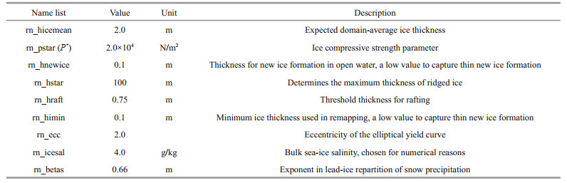
In this formula, the parameters affecting the strength of sea ice are mainly P* and Crhg. Previous studies have explored the impacts of P* on the Arctic sea ice by model sensitivity experiments. Docquier et al. (2017) found that higher values of P* generally result in lower sea ice deformation and lead to lower sea ice thickness, based on the NEMO-LIM model. They concluded that P* has limited influences in mean sea ice concentration and no single value of P* is the best option for reproducing the observed Arctic sea ice. Based on NEMO-CICE coupled ice-ocean prediction system, Chikhar et al. (2019) showed that the increase of P* value will enhance the ice compressive strength and slow down the sea ice drift speed in summer, and reduce the model deviation compared with observation. However, the decrease of sea ice velocity will exacerbate the simulation bias in fall and winter. In contrast, the influence of changing Crhg on the compressive strength is relatively small in cold seasons when the sea ice concentration is close to 100%. Chikhar et al. (2019) proposed that it would be more suitable to change the ice compressive strength by Crhg parameter rather than P* parameter because of the relationship between the sea ice coverage area and Crhg parameter. Therefore, two model sensitivity experiments were designed based on NAPA1/4 to explore the influences of sea ice compressive strength on ice drift velocity, sea ice concentration, and thickness. The experiments involved two different Crhg values of 20 and 5, corresponding to NAPA1/4 (A) and NAPA1/4 (B). This setting is referenced to Chikhar et al. (2019) and Sumata et al. (2019) based on the model of NEMO-CICE and NAOSIM (North Atlantic/Arctic Ocean Sea-Ice Model developed at the Alfred Wegener Institute). In their sensitivity experiments, the values of Crhg range from 5 to 20. Other main sea ice parameters are shown in Table 1.
Sea ice area is a measure of the surface area of the Arctic Ocean covered by sea ice including the influence of sea ice concentration. Sea ice area is the integral sum of the product of ice concentration and area of all grid cells with at least 15% ice concentration (Dong et al., 2021). There are strong correlation between NAPA1/4 (A) and CDR as well as that between NAPA1/4 (B) and CDR, the correlation coefficients are R=0.97 (P < 0.001) and R=0.98 (P < 0.001), respectively. Overall, NAPA1/4 (A) and NAPA1/4 (B) reproduce the consistent variation in annual averaged sea ice area and catch the special years of minimum sea ice area in 2007 and 2012 in the Arctic Ocean with that displayed by the CDR dataset as shown in Fig. 2. The root mean square errors (RMSEs) are 0.25×10⁶ km2 and 0.18×10⁶ km2, correspondingly. NAPA1/4 (B) is more consistent with satellite observed results and has a lower deviation, especially after the year of 2007.

|
| Fig.2 Time series of the annual averaged sea ice area between 65°N and 90°N from 1994 to 2015 |
The cost function (CF) is further applied to quantify the "goodness of fit" between satellite observations and model results. CF is the sum of the absolute values of the differences between model and observation results, divided by the product of the number and the standard deviation of observations (Radach and Moll, 2006). The formula of CF is defined as follow:
 (2)
(2)where M represents model results, D derives from satellite observations, n is the number of all satellite observations, σD is the standard deviation of observations. The criteria for CF are as follows: 0–1 (excellent/very good), 1–2 (good), 2–3 (reasonable), and > 3 (poor/bad) (Radach and Moll, 2006). The CF value for annual averaged sea ice area from the period of 1994 to 2015 between CDR and NAPA1/4 (A) is 0.56, as well as that the CF value between CDR and NAPA1/4 (B) is 0.41. These suggest that NAPA1/4 (B) model presents a better performance in simulating interannual variations in Arctic sea ice area compared with NAPA1/4 (A).
3.2 Ice condition in melting seasonThe outputs of NAPA1/4 (A) and NAPA1/4 (B) covered the same period from 1993 to 2015. Note that NAPA1/4 (A) has been in use and adequately evaluated in the Arctic continental shelf seas (Luo et al., 2020; Zhang et al., 2020; Dong et al., 2021). For example, in the Bering Strait region, the model simulated dates of open-water onset (earliest date when regional averaged ice concentration reached below 30%) matched well with the CDR satellite observations (R=0.94) (Luo et al., 2020). In the Beaufort and the Chukchi Sea, the mean bias of modeled ice thickness and drill-hole observations was found to be 0.1 m over 2002–2004, and the yearly summer open-water area agreed well with satellite observations (R=0.87) with the presence of extremely low ice conditions in 1998, 2008, 2012, and 2016 (Zhang et al., 2020). In the Kara Sea, the modeled sea ice coverage exhibited consistent interannual variations (R=0.96) with CDR observational results (Dong et al., 2021). However, in the central Arctic Ocean, the results of NAPA1/4 (A) exhibited significant differences from observations. In some summers, such as those of the years 1996, 2002, 2008, and 2013, the simulated sea ice had a much lower concentration and melted faster (Fig. 3e–h) compared with CDR observations (Fig. 3a–d). In particular, the summer of 1996 presented a much lower ice concentration in the central Arctic Ocean than in the surrounding areas. By reducing the value of the Crhg parameter, the performance of NAPA1/4 (B) was significantly improved (Fig. 3i–l). The sea ice concentration of the central Arctic Ocean increased, and the spatial distribution was more consistent with that based on satellite observations. The RMSE between the simulated and observed sea ice concentration averaged over the central Arctic Ocean (the region outlined in black) was reduced by 15%.

|
| Fig.3 Arctic sea ice concentration in August 1996, 2002, 2008, and 2013 based on CDR (a–d), NAPA1/4 (A) (e–h), and NAPA1/4 (B) (i–l), respectively, with sea ice edge defined by a sea ice concentration of 15% The region outlined in black represents the central Arctic Ocean. |
Taking August 1996 as an example, the causes of the differences between the sea ice conditions simulated by the two sensitivity experiments are analyzed. The parameterization of sea ice compressive strength in the model rheology has a significant effect on simulated ice drift (Chikhar et al., 2019). Sea ice drift reflects the characteristics of large-scale spatial motion of sea ice, affecting the spatial distribution of sea ice. Both NAPA1/4 (A) and NAPA1/4 (B) exhibited the main spatial patterns of sea ice drift, such as transpolar ice drift and anticyclone circulation in the Beaufort Sea (Fig. 4a–b). Among the channels between the Arctic Ocean and other oceans, sea ice outflowing through the Fram Strait dominated the entire export of Arctic sea ice, while a small portion of the sea ice was transported through the Canadian Arctic Archipelago. This is consistent with the findings based on the observations of Arctic sea ice motion by NSIDC (Wei et al., 2019).

|
| Fig.4 Mean sea ice drift velocity (color shading, in cm/s) and directions (arrows) in NAPA1/4 (A) (a) and NAPA1/4 (B) (b), and their difference (NAPA1/4 (B) - NAPA1/4 (A)) (c) in August of 1996 The upper colorbar corresponds to (a) and (b), the lower one corresponds to (c). The region outlined in black represents the central Arctic Ocean. |
The differences in sea ice drifting speed between NAPA1/4 (A) and NAPA1/4 (B) are presented in Fig. 4c. The speed was generally smaller in NAPA1/4 (B) than in NAPA1/4 (A) in multiyear ice areas, such as the areas adjacent to Greenland and the northern Canadian Arctic Archipelago, as well as in some seasonal sea ice areas, such as the Laptev Sea and the East Siberian Sea. The sea ice output velocity through the Fram Strait was lower (4.50 cm/s) in NAPA1/4 (B) than that in NAPA1/4 (A) (9.19 cm/s). Based on the differences in the sea ice drift velocity vectors, NAPA1/4 (B) obtained a reduced ice export of sea ice through the Fram Strait and slower ice movement from the central Arctic to the multiyear ice region (Fig. 4c). Consequently, more sea ice remained in the central Arctic Ocean, contributing to the increased ice concentration. The model sensitivity experiments show consistent results with Chikhar et al. (2019) who suggests that decreasing Crhg lowers the modeled summer ice velocity and reduces the model bias based on NEMO-CICE.
Variations in sea ice thickness are determined by dynamic and thermodynamic processes (Rigor et al., 2002; Lindsay and Zhang, 2005; Hu et al., 2018). The thermodynamic and dynamic effects are interrelated (Holland et al., 1993). In our model, the thermodynamic contribution represents the vertical heat fluxes through the atmosphere-ice and ice-ocean interfaces, determining the ice freezing and melting. The dynamic processes include sea ice movement (advection and convergence/divergence) and mechanical redistribution (rafting and ridging). To disentangle the contributions of thermodynamic and dynamic processes to the change of summer Arctic sea ice thickness simulated between NAPA 1/4 (A) and NAPA 1/4 (B), we apply the methodology of Zhang et al. (2020). The thermodynamic contribution is estimated based on model diagnostic results. The dynamic contribution is defined as the total ice thickness changes minus thermodynamic contribution.
The thermodynamic and dynamic contributions to ice thickness changes in August of 1996 based on NAPA1/4 (A) and NAPA1/4 (B) in Fig. 5. Negative (positive) values indicate the rate of sea ice decrease (increase). The effects of dynamic processes on sea ice thickness variation widely differed between the two experiments, especially in the central Arctic Ocean with ice convergence in NAPA1/4 (A) but ice divergence in NAPA1/4 (B) (Fig. 5a–b). The entire Arctic sea ice is subject to melting in August due to thermodynamic processes (Fig. 5c–d). Over the central Arctic Ocean, large differences were observed between the results of the two experiments, with NAPA1/4 (B) presenting weaker thermodynamical ice loss than NAPA1/4 (A). In NAPA1/4 (B), the dynamic and thermodynamic processes exhibited the opposite effects on changes in ice thickness. Consequently, larger ice thickness and higher ice concentration were simulated in NAPA1/4 (B). On the contrary, in NAPA1/4 (A), the dynamic and thermodynamic processes played the same role in reducing sea ice thickness, thus accelerating both ice thinning and retreat in the central Arctic Ocean.

|
| Fig.5 Rate of sea ice increase and decrease in August of 1996 based on NAPA1/4 (A) (a, c) and NAPA1/4 (B) (b, d) The upper and lower panels respectively represent the contributions of dynamic and thermodynamic processes to sea ice thickness variation. Negative (positive) values indicate the rate of sea ice decrease (increase). The region outlined in black represents the central Arctic Ocean. |
The contribution ratios of dynamic and thermodynamic processes were quantitatively analyzed in the central Arctic Ocean (outlined in black in Fig. 1) through the rates of sea ice increase and decrease. Taking dynamic processes as an example, the regional averaged thickness change and contribution ratio are calculated as follows:
 (3)
(3)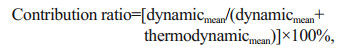 (4)
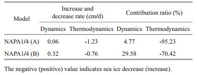
(4)where e1ti and e2ti represent the length and width of a cell grid, respectively; dynamicsi represents the ice thickness change induced by dynamic processes in each cell grid. The lower Crhg in NAPA1/4 (B) leads to higher sea ice compressive strength than in NAPA1/4 (A). Consequently, a lower contribution (70.42%) of thermodynamic processes to sea ice retreat was estimated, compared with NAPA1/4 (A) (95.23%) (Table 2). This can be attributed to the lower degree of deformation and fracture of sea ice. Meanwhile, dynamic processes contributed to 30% of sea ice growth in NAPA1/4 (B), which was significantly higher than that in NAPA1/4 (A) (5%). Accordingly, averaged sea ice thickness changes of 0.32 cm/d and 0.06 cm/d were estimated, respectively. Combined with the sea ice velocity field, ice export through the Fram Strait was decreased in NAPA1/4 (B) and more ice was constrained in the central Arctic Ocean, driven by the dynamic processes. Consequently, NAPA1/4 (B) simulated a higher ice concentration than NAPA1/4 (A).
|
CryoSat-2/SMOS provides relatively reliable sea ice thickness data after 2010. A previous study suggested that CryoSat-2/SMOS significantly reduces the uncertainty of single-sensor products and improves the accuracy of sea ice thickness inversion (Ricker et al., 2017). Therefore, the simulated sea ice thickness from 2011 to 2015 was compared with CryoSat-2/SMOS satellite products (Figs. 6–7).

|
| Fig.6 Spatial distribution of sea ice thickness in March from 2011 to 2015 based on CryoSat-2/SMOS (a–e), NAPA1/4 (A) (f–j), and NAPA1/4 (B) (k–o) |

|
| Fig.7 Same as Fig. 6, but for October |
Figure 6 shows the sea ice thickness simulated by both NAPA and observed by CryoSat-2/SMOS in March from 2011 to 2015. Both experiments reproduced the general features of thicker ice in the north of the Canadian Arctic Archipelago and Greenland as revealed by the observations. Simulated ice thickness in the central Arctic Ocean was much larger in NAPA1/4 (A) (Fig. 6f–j) than that revealed by CryoSat-2/SMOS observations (Fig. 6a–e), with the maximum bias exceeding 1 m (Fig. 8a–e). Meanwhile, NAPA1/4 (B) presented an improved representation of ice thickness (Fig. 6k–o). Sea ice in the Canadian Basin was significantly thinner and closer to the CryoSat-2/SMOS products than NAPA1/4 (A) (Fig. 8k–o). In both model experiments, ice thickness in the Beaufort Sea was generally overestimated, while that in the north of Greenland and the Canadian Arctic Archipelago was underestimated. These features have also been documented in PIOMAS (Schweiger et al., 2011) and the AOMIP models (Johnson et al., 2012).

|
| Fig.8 Differences of sea ice thickness (cm) in March and October from 2011 to 2015, between NAPA1/4 (A) (a–j) and CryoSat-2/SMOS as well as that of NAPA1/4 (B) and CryoSat-2/SMOS (k–t) |
Figure 7 shows ice thickness in October based on the model and CryoSat-2/SMOS results. NAPA1/4 (B) provided similar interannual variations with thicker ice near the Canadian Arctic Archipelago in 2013 and 2014 and a larger open water area in the Beaufort Sea in 2012, consistent with observations (Fig. 7k–o). These interannual features were less prominent in NAPA1/4 (A) (Fig. 7f–j). In both experiments, ice thickness in the Laptev-East Siberian seas in autumn was overestimated (Fig. 8). This bias may be attributable to the lack of a landfast ice parameterization in the model (Johnson et al., 2012). In addition, the two experiments underestimated sea ice thickness in the Arctic Atlantic Sector near the Fram Strait. This phenomenon has also been reported for many reanalysis systems (Chevallier et al., 2017). In NAPA1/4 (B), the thickness of thick sea ice of the Canada Basin was reduced (Fig. 8p–t) which is similar to that in March. This is consistent with Docquier et al. (2017) who suggests that higher initial compressive strength leads to lower ice thickness through the whole year by adjusting P* based on NEMO-LIM due to lower deformation rates preventing ice from thickening via ridging and rafting. On the other hand, weaker compressive strength renders the ice prone to ridging, resulting in more leads. As these open water areas freeze in autumn and winter, new ice is generated (Uotila et al., 2012). With a lower sea ice compressive strength, NAPA1/4 (A) simulates thicker sea ice than observed (Fig. 8f–j). By increasing the sea ice compressive strength, NAPA1/4 (B) simulates thinner and therefore more realistic sea ice thicknesses.
We investigated the time evolution of the area covered by sea ice within specific ice classes to gain deeper insight into ice thickness variations. The ice classes we applied were similar to those used by Chevallier and Salas-Mélia (2012): 0–0.5 m, 0.5–0.9 m, 0.9–1.5 m, 1.5–2.5 m, 2.5–4 m, and > 4 m. The time series of monthly sea ice area for each thickness class in March and October during 1994–2015 are presented in Fig. 9 Both experiments presented a similar trend of decreasing the proportion of thick ice (> 2.5 m) in both months, and increasing proportions of medium ice (0.9–2.5 m) in March and thin ice (< 0.9 m) in October. The model reflected extreme years (2007 and 2012), during which the sea ice area was low in October, as recorded by historical observations (Overland and Wang, 2013). After 2007, NAPA1/4 (B) presented a larger area of sea ice with a thickness of 1.5–2.5 m in March, and the proportion of thick ice with a thickness greater than 2.5 m was declined (Fig. 9a & c). In October, sea ice with a thickness of 0.9–2.5 m accounted for a considerable proportion of the total area, much larger than that simulated by NAPA1/4 (A) (Fig. 9b & d), and the proportion of areas of sea ice thicker than 2.5 m was decreased. In March, the proportion of sea ice cover thinner than 0.9 m simulated by NAPA1/4 (B) was equivalent to that by NAPA1/4 (A), while in October, thin ice coverage was substantially increased in NAPA1/4 (B). Overall, enhancing the ice compressive strength by reducing the parameter of Crhg has a stronger impact on thicker ice, reducing the proportion of multiyear ice in the freezing season.

|
| Fig.9 Area covered by sea ice of following classes as simulated by NAPA1/4 (A) (a–b) and NAPA1/4 (B) (c–d): 0–0.5 m, 0.5–0.9 m, 0.9–1.5 m, 1.5–2.5 m, 2.5–4.0 m, above 4 m |
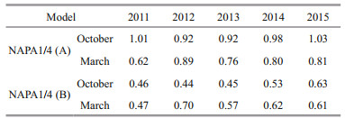
Previous study evaluated ORA-IP (Ocean ReAnalyses Intercomparison Project) reanalyzed sea ice thickness data using ICESat (Ice, Cloud, and land Elevation Satellite) observation results (Chevallier et al., 2017). The RMSEs varied in the ranges of 0.93– 1.82 m and 0.92–1.61 m in winter-spring (February–March 2004, 2005, 2006, and March–April 2007) and autumn (October–November 2004, 2005, 2006, and 2007), respectively. In this study, the averaged RMSEs between the simulated and CryoSat-2/SMOS ice thickness (Table 3) in October over 2011–2015 were 0.50 m in NAPA1/4 (B) and 0.97 m in NAPA1/4 (A). The averaged RMSEs for March were 0.60 m and 0.78 m, correspondingly. Compared with NAPA1/4 (A), NAPA1/4 (B) reflects reductions by 23.1% and 48.5% respectively in March and October. NAPA1/4 (B) presented comparable RMSEs to the ocean and sea ice models in ORA-IP. NAPA1/4 (B) presented comparable RMSEs to the ocean and sea ice models in ORA-IP.
|
Based on satellite observed ice thickness from CryoSat-2/SMOS, cost function (CF) values of ice thickness from NAPA1/4 (A) and NAPA1/4 (B) were further computed in March and October from 2011 to 2015 (Fig. 10). The results show that CF values are less than 1 except for October in the years of 2011 and 2015 in NAPA1/4 (A). NAPA1/4 (B) has smaller CF values in both March and October showing the better performance in the simulation of sea ice thickness in the Arctic Ocean. The still existing discrepancies between NAPA1/4 (B) and satellite observations, including sea ice concentration and thickness, are largely due to the uncertainties associated with sea ice parameterizations and that transferred from the physical fields. In the high-latitude oceans, some meso- and submeso-scale physical features are beyond the ability of the medium resolution NAPA1/4 model to resolve.

|
| Fig.10 Cost function (CF) values of ice thickness from NAPA1/4 (A) and NAPA1/4 (B) based on CryoSat-2/SMOS in March (a) and October (b) from 2011 to 2015 The dashed line represents CF=1. |
This study focused on the influences of ice strength decay constant parameter (Crhg) on the simulation of the Arctic sea ice based on the coupled ocean and sea ice model (NAPA1/4). Two sensitivity experiments were performed with different values of Crhg (Crhg=20 and 5, corresponding to NAPA1/4 (A) and NAPA1/4 (B)).
The lower Crhg in NAPA1/4 (B) leads to higher sea ice compressive strength than in NAPA1/4 (A) and improves hindcast simulation of sea ice conditions. Particularly, the underestimated summer sea ice concentration in NAPA1/4 (A) was increased in NAPA1/4 (B) in the central Arctic Ocean. In this region, the thermodynamic contribution to sea ice melting was found to reduce with increased compressive strength, while the dynamic contribution to sea ice growth was found to increase in NAPA1/4 (B). Results of sea ice drift in NAPA1/4 (B) further indicated that sea ice is more likely to be retained in the central Arctic Ocean. This led to a higher summer ice concentration there compared with NAPA1/4 (A).
Additionally, lowering Crhg improved the spatial distribution of sea ice thickness, as confirmed through comparison with CryoSat-2/SMOS satellite-based results after 2010. The proportion of areas with thicker ice cover decreased in NAPA1/4 (B), especially in multiyear ice regions in the Canada Basin and northern Greenland. The RMSEs between NAPA1/4 (B) and observation results in March and October were respectively 0.5 m and 0.6 m, reflecting reductions by 23.1% and 48.5%, compared to NAPA1/4 (A). NAPA1/4 (B) presented comparable RMSEs to the world's widely used ocean and sea ice models.
NAPA1/4 (B) enhanced the ice compressive strength, thus improving its performance in simulating the spatial distribution of sea ice. By setting an appropriate ice compressive strength, underestimated thin ice can be thickened and overestimated thick ice can be thinned. The improvement of sea ice simulation conditions will provide an essential foundation for future research on the response of the primary production and biogeochemical cycling to sea ice changes in related biological hotspots such as the Chukchi Borderland. We expect the findings of this study can provide some guidance for parameter adjustment in the coupled ocean and sea ice models. We also expect that the parameterizations of sea ice compressive strength will be improved based on more available observed field tests.
5 DATA AVAILABILITY STATEMENTThe datasets generated and/or analyzed during the current study are available from the corresponding author on reasonable request.
6 ACKNOWLEDGMENTWe are grateful to the NEMO (Nucleus for European Modelling of the Ocean) development team for providing the state-of-the-art ocean modeling framework. Climate Data Record of Passive Microwave Sea Ice Concentration (Version 4) was derived from NSIDC (National Snow and Ice Data Centre of the USA National Oceanic and Atmospheric Administration, https://nsidc.org/data/G02202/). The merging of CryoSat-2 and SMOS data was funded by the ESA project SMOS & CryoSat-2 Sea Ice Data Product Processing and Dissemination Service and data were obtained from https://www.meereisportal.de (grant No.: REKLIM-2013-04).
Bai Y C, Sicre M A, Chen J F, et al. 2019. Seasonal and spatial variability of sea ice and phytoplankton biomarker flux in the Chukchi Sea (western Arctic Ocean). Progress in Oceanography, 171: 22-37.
DOI:10.1016/j.pocean.2018.12.002 |
Bouillon S, Fichefet T, Legat V, et al. 2013. The elastic-viscous-plastic method revisited. Ocean Modelling, 71: 2-12.
DOI:10.1016/j.ocemod.2013.05.013 |
Cavalieri D J, Gloersen P, Campbell W J. 1984. Determination of sea ice parameters with the NIMBUS 7 SMMR. Journal of Geophysical Research: Atmospheres, 89(D4): 5355-5369.
DOI:10.1029/JD089iD04p05355 |
Cavalieri D J, Parkinson C L. 2012. Arctic sea ice variability and trends, 1979-2010. The Cryosphere, 6(4): 881-889.
DOI:10.5194/tc-6-881-2012 |
Chevallier M, Salas-Mélia D. 2012. The role of sea ice thickness distribution in the Arctic sea ice potential predictability: a diagnostic approach with a coupled GCM. Journal of Climate, 25(8): 3025-3038.
DOI:10.1175/JCLI-D-11-00209.1 |
Chevallier M, Smith G C, Dupont F, et al. 2017. Intercomparison of the arctic sea ice cover in global ocean-sea ice reanalyses from the ORA-IP project. Climate Dynamics, 49(3): 1107-1136.
DOI:10.1007/s00382-016-2985-y |
Chikhar K, Lemieux J F, Dupont F, et al. 2019. Sensitivity of ice drift to form drag and ice strength parameterization in a coupled ice-ocean model. Atmosphere-Ocean, 57(5): 329-349.
DOI:10.1080/07055900.2019.1694859 |
Comiso J C. 1986. Characteristics of Arctic winter sea ice from satellite multispectral microwave observations. Journal of Geophysical Research: Oceans, 91(C1): 975-994.
DOI:10.1029/JC091iC01p00975 |
Dai A G, Trenberth K E. 2002. Estimates of freshwater discharge from continents: latitudinal and seasonal variations. Journal of Hydrometeorology, 3(6): 660-687.
DOI:10.1175/1525-7541(2002)003<0660:EOFDFC>2.0.CO;2 |
Docquier D, Massonnet F, Barthélemy A, et al. 2017. Relationships between Arctic sea ice drift and strength modelled by NEMO-LIM3.6. The Cryosphere, 11(6): 2829-2846.
DOI:10.5194/tc-11-2829-2017 |
Dong C M, Nie H T, Luo X F, et al. 2021. Mechanisms for the link between onset and duration of open water in the Kara Sea. Acta Oceanologica Sinica, 40(11): 119-128.
|
Dussin R, Barnier B, Brodeau L et al. 2016. The making of the DRAKKAR FORCING SET DFS5. DRAKKAR/MyOcean Report 01-04-16. https://www.drakkar-ocean.eu/publications/reports/report_DFS5v3_April2016.pdf.
|
Ferry N, Parent L, Garric G et al. 2012. GLORYS2V1 global ocean reanalysis of the altimetric era (1992-2009) at meso scale. Mercator Quarterly Newsletter 44, January 2012, 29-39. http://www.mercator-ocean.fr/eng/actualites-agenda/newsletter.
|
Francis J A, Vavrus S J. 2012. Evidence linking Arctic amplification to extreme weather in mid-latitudes. Geophysical Research Letters, 39(6).
DOI:10.1029/2012GL051000 |
Hibler III W D. 1979. A dynamic thermodynamic sea ice Model. Journal of Physical Oceanography, 9(4): 815-846.
DOI:10.1175/1520-0485(1979)009<0815:ADTSIM>2.0.CO;2 |
Hirawake T, Uchida M, Abe H, et al. 2021. Response of Arctic biodiversity and ecosystem to environmental changes: findings from the ArCS project. Polar Science, 27: 100533.
DOI:10.1016/j.polar.2020.100533 |
Holland D M, Mysak L A, Manak D K, et al. 1993. Sensitivity study of a dynamic thermodynamic sea ice model. Journal of Geophysical Research: Oceans, 98(C2): 2561-2586.
DOI:10.1029/92JC02015 |
Holland M M, Stroeve J. 2011. Changing seasonal sea ice predictor relationships in a changing Arctic climate. Geophysical Research Letters, 38(18): L18501.
DOI:10.1029/2011GL049303 |
Honda M, Inoue J, Yamane S. 2009. Influence of low Arctic sea-ice minima on anomalously cold Eurasian winters. Geophysical Research Letters, 36(8): L08707.
DOI:10.1029/2008GL037079 |
Hu X M, Sun J F, Chan T O, et al. 2018. Thermodynamic and dynamic ice thickness contributions in the Canadian Arctic Archipelago in NEMO-LIM2 numerical simulations. The Cryosphere, 12(4): 1233-1247.
DOI:10.5194/tc-12-1233-2018 |
Huang W F, Lei R B, Han H W, et al. 2016. Physical structures and interior melt of the central Arctic sea ice/snow in summer 2012. Cold Regions Science and Technology, 124: 127-137.
DOI:10.1016/j.coldregions.2016.01.005 |
Johnson M, Proshutinsky A, Aksenov Y, et al. 2012. Evaluation of Arctic sea ice thickness simulated by Arctic Ocean Model Intercomparison Project models. Journal of Geophysical Research: Oceans, 117(C8): C00D13.
DOI:10.1029/2011JC007257 |
Kȩdra M, Moritz C, Choy E S, et al. 2015. Status and trends in the structure of Arctic benthic food webs. Polar Research, 34(1): 23775.
DOI:10.3402/polar.v34.23775 |
Kim J G, Hunke E C, Lipscomb W H. 2006. Sensitivity analysis and parameter tuning scheme for global sea-ice modeling. Ocean Modelling, 14(1-2): 61-80.
|
Kreyscher M, Harder M, Lemke P, et al. 2000. Results of the Sea Ice Model Intercomparison Project: evaluation of sea ice rheology schemes for use in climate simulations. Journal of Geophysical Research, 105(C5): 11299-11320.
DOI:10.1029/1999jc000016 |
Kwok R, Rothrock D A. 2009. Decline in Arctic sea ice thickness from submarine and ICESat records: 1958-2008. Geophysical Research Letters, 36(15): L15501.
DOI:10.1029/2009GL039035 |
Kwok R, Spreen G, Pang S. 2013. Arctic sea ice circulation and drift speed: decadal trends and ocean currents. Journal of Geophysical Research: Oceans, 118(5): 2408-2425.
DOI:10.1002/jgrc.20191 |
Lei R B, Xie H J, Wang J, et al. 2015. Changes in sea ice conditions along the Arctic Northeast Passage from 1979 to 2012. Cold Regions Science and Technology, 119: 132-144.
DOI:10.1016/j.coldregions.2015.08.004 |
Lindsay R W, Zhang J. 2005. The thinning of Arctic sea ice, 1988-2003: have we passed a tipping point?. Journal of Climate, 18(22): 4879-4894.
DOI:10.1175/JCLI3587.1 |
Lipscomb W H, Hunke E C, Maslowski W, et al. 2007. Ridging, strength, and stability in high-resolution sea ice models. Journal of Geophysical Research: Oceans, 112(3): C03S91.
DOI:10.1029/2005JC003355 |
Locarnini R A, Mishonov A V, Antonov J I et al. 2013. World Ocean Atlas 2013, Volume 1: Temperature. Levitus S, Ed. Mishonov A, Technical Ed. NOAA Atlas NESDIS 73, 40p, https://www.ncei.noaa.gov/data/oceans/woa/WOA13/DOC/woa13_vol1.pdf.
|
Luo X F, Hu X M, Nie H T, et al. 2019. Evaluation of hindcast simulation with the ocean and sea-ice model covering the Arctic and adjacent oceans. Acta Oceanologica Sinica, 41(9): 1-12.
(in Chinese with English abstract) DOI:10.3969/j.issn.0253-4193.2019.09.001 |
Luo X F, Wang Y L, Lu Y Y, et al. 2020. A 4-month lead predictor of open-water onset in Bering Strait. Geophysical Research Letters, 47(17): e2020GL089573.
DOI:10.1029/2020GL089573 |
Madec G. 2008. NEMO Ocean Engine, Note du Pôle de Modélisation. Institut Pierre-Simon Laplace (IPSL), France.
|
Madec G, Imbard M. 1996. A global ocean mesh to overcome the North Pole singularity. Climate Dynamics, 12(6): 381-388.
DOI:10.1007/BF00211684 |
Marchi S, Fichefet T, Goosse H. 2020. Respective influences of perturbed atmospheric and ocean-sea ice initial conditions on the skill of seasonal Antarctic sea ice predictions: a study with NEMO3.6-LIM3. Ocean Modelling, 148: 101591.
DOI:10.1016/j.ocemod.2020.101591 |
Maslanik J A, Fowler C, Stroeve J, et al. 2007. A younger, thinner Arctic ice cover: increased potential for rapid, extensive sea-ice loss. Geophysical Research Letters, 34(24): L24501.
DOI:10.1029/2007GL032043 |
Maykut G A, Untersteiner N. 1971. Some results from a time-dependent thermodynamic model of sea ice. Journal of Geophysical Research, 76(6): 1550-1575.
DOI:10.1029/jc076i006p01550 |
Meier W, Fetterer F, Duerr R et al. 2017. NOAA/NSIDC climate data record of passive microwave sea ice concentration, version 3. National Snow and Ice Data Center, Boulder, Colorado USA.
|
Miller P A, Laxon S W, Feltham D L, et al. 2006. Optimization of a sea ice model using basinwide observations of Arctic sea ice thickness, extent, and velocity. Journal of Climate, 19(7): 1089-1108.
DOI:10.1175/JCLI3648.1 |
Molines J M, Barnier B, Penduff T et al. 2007. Definition of the Interannual Experiment ORCA025-G70, 1958-2004. Laboratoire des Ecoulements Geophysiques et Industriels, Grenoble, France.
|
Moreno-Chamarro E, Ortega P, Massonnet F. 2020. Impact of the ice thickness distribution discretization on the sea ice concentration variability in the NEMO3.6-LIM3 global ocean-sea ice model. Geoscientific Model Development, 13(10): 4773-4787.
DOI:10.5194/gmd-13-4773-2020 |
Nghiem S V, Rigor I G, Perovich D K, et al. 2007. Rapid reduction of Arctic perennial sea ice. Geophysical Research Letters, 34(19): L19504.
DOI:10.1029/2007GL031138 |
Overland J E, Wang M Y. 2013. When will the summer Arctic be nearly sea ice free?. Geophysical Research Letters, 40(10): 2097-2101.
DOI:10.1002/grl.50316 |
Pemberton P, Löptien U, Hordoir R, et al. 2017. Sea-ice evaluation of NEMO-Nordic 1.0: a NEMO-LIM3.6-based ocean-sea-ice model setup for the North Sea and Baltic Sea. Geoscientific Model Development, 10(8): 3105-3123.
DOI:10.5194/gmd-10-3105-2017 |
Pizzolato L, Howell S E L, Dawson J, et al. 2016. The influence of declining sea ice on shipping activity in the Canadian Arctic. Geophysical Research Letters, 43(23): 12146-12154.
DOI:10.1002/2016GL071489 |
Prasad S, Zakharov I, Bobby P, et al. 2015. The implementation of sea ice model on a regional high-resolution scale. Ocean Dynamics, 65(9-10): 1353-1366.
DOI:10.1007/s10236-015-0877-z |
Radach G, Moll A. 2006. Review of three-dimensional ecological modelling related to the North Sea shelf system. Part Ⅱ: model validation and data needs. In: Gibson R N, Atkinson R J A, Gordon J D M eds. Oceanography and Marine Biology: an Annual Review. CRC Press, Boca Raton, p. 1-60, https://doi.org/10.1201/9781420006391.
|
Ricker R, Hendricks S, Kaleschke L, et al. 2017. A weekly Arctic sea-ice thickness data record from merged CryoSat-2 and SMOS satellite data. The Cryosphere, 11(4): 1607-1623.
DOI:10.5194/tc-11-1607-2017 |
Rigor I G, Wallace J M, Colony R L. 2002. Response of sea ice to the Arctic oscillation. Journal of Climate, 15(18): 2648-2663.
DOI:10.1175/1520-0442(2002)015<2648:ROSITT>2.0.CO;2 |
Rothrock D A. 1975. The energetics of the plastic deformation of pack ice by ridging. Journal of Geophysical Research, 80(33): 4514-4519.
DOI:10.1029/JC080i033p04514 |
Rousset C, Vancoppenolle M, Madec G, et al. 2015. The Louvain-La-Neuve sea ice model LIM3.6: global and regional capabilities. Geoscientific Model Development, 8(10): 2991-3005.
DOI:10.5194/gmd-8-2991-2015 |
Schweiger A, Lindsay R, Zhang J L, et al. 2011. Uncertainty in modeled Arctic sea ice volume. Journal of Geophysical Research: Oceans, 116(C8): C00D06.
DOI:10.1029/2011JC007084 |
Semtner A J Jr. 1976. A model for the thermodynamic growth of sea ice in numerical investigations of climate. Journal of Physical Oceanography, 6(3): 379-389.
DOI:10.1175/1520-0485(1976)006<0379:amfttg>2.0.co;2 |
Stroeve J C, Markus T, Boisvert L, et al. 2014. Changes in Arctic melt season and implications for sea ice loss. Geophysical Research Letters, 41(4): 1216-1225.
DOI:10.1002/2013GL058951 |
Sumata H, Kauker F, Karcher M, et al. 2019. Covariance of optimal parameters of an arctic sea ice-ocean model. Monthly Weather Review, 147(7): 2579-2602.
DOI:10.1175/MWR-D-18-0375.1 |
Timco G W, Frederking R M W. 1991. Seasonal compressive strength of Beaufort sea ice sheets. In: Jones S J, Tillotson J, McKenna R F et al eds. Ice-Structure Interaction. Springer, New York. p. 267-282.
|
Ungermann M, Tremblay L B, Martin T, et al. 2017. Impact of the ice strength formulation on the performance of a sea ice thickness distribution model in the Arctic. Journal of Geophysical Research: Oceans, 122(3): 2090-2107.
DOI:10.1002/2016JC012128 |
Uotila P, Iovino D, Vancoppenolle M, et al. 2017. Comparing sea ice, hydrography and circulation between NEMO3.6 LIM3 and LIM2. Geoscientific Model Development, 10(2): 1009-1031.
DOI:10.5194/gmd-10-1009-2017 |
Uotila P, O'Farrell S, Marsland S J, et al. 2012. A sea-ice sensitivity study with a global ocean-ice model. Ocean Modelling, 51: 1-18.
DOI:10.1016/j.ocemod.2012.04.002 |
Vancoppenolle M, Fichefet T, Goosse H, et al. 2009. Simulating the mass balance and salinity of Arctic and Antarctic sea ice. 1. Model description and validation. Ocean Modelling, 27(1-2): 33-53.
DOI:10.1016/j.ocemod.2008.10.005 |
Wang Q K, Li Z J, Lei R B, et al. 2018. Estimation of the uniaxial compressive strength of Arctic sea ice during melt season. Cold Regions Science and Technology, 151: 9-18.
DOI:10.1016/j.coldregions.2018.03.002 |
Wang Y L, Luo X F, Zhang Y L, et al. 2019. Heat budget analysis during the ice-melting season in the Chukchi Sea based on a model simulation. Chinese Science Bulletin, 64(33): 3485-3497.
DOI:10.1360/N972019-00322 |
Wei J F, Zhang X D, Wang Z M. 2019. Reexamination of Fram Strait sea ice export and its role in recently accelerated Arctic sea ice retreat. Climate Dynamics, 53(3-4): 1823-1841.
DOI:10.1007/s00382-019-04741-0 |
Zhang Y L, Wei H, Lu Y Y, et al. 2020. Dependence of Beaufort Sea low ice condition in the summer of 1998 on ice export in the prior winter. Journal of Climate, 33(21): 9247-9259.
DOI:10.1175/JCLI-D-19-0943.1 |
Zheng Z J, Wei H, Luo X F, et al. 2021. Mechanisms of persistent high primary production during the growing season in the Chukchi Sea. Ecosystems, 24(4): 891-910.
DOI:10.1007/s10021-020-00559-8 |
Zweng M M, Reagan J R, Antonov J I et al. 2013. World Ocean Atlas 2013. Volume 2: Salinity. Levitus S, Ed. Mishonov A, Technical Ed. NOAA Atlas NESDIS 74, 39p, http://data.nodc.noaa.gov/woa/WOA13/DOC/woa13_vol2.pdf.
|