 2022, Vol. 40
Institute of Oceanology, Chinese Academy of Sciences
Article Information
- ZHANG Huaguo, WANG Juan, LI Dongling, FU Bin, LOU Xiulin, WU Ziyin
- Reconstruction of large complex sand-wave bathymetry with adaptive partitioning combining satellite imagery and sparse multi-beam data
- Journal of Oceanology and Limnology, 40(5): 1924-1936
- http://dx.doi.org/10.1007/s00343-021-1216-5
Article History
- Received Jul. 5, 2021
- accepted in principle Aug. 31, 2021
- accepted for publication Oct. 28, 2021


2 Key Laboratory of Submarine Geosciences, Second Institute of Oceanography, Ministry of Natural Resources, Hangzhou 310012, China;
3 School of Oceanography, Shanghai Jiao Tong University, Shanghai 200240, China
Shallow marine sand waves are widely distributed in tidal environments (Allen, 1982). Studies of shallow-water sand-wave topography are of great significance for use in coastal protection (Whitehouse et al., 1998), ensuring maritime safety (Katoh et al., 1998), when laying submarine pipelines, and for drilling platform construction programs (Morelissen et al., 2003).
Current research focusing on sand waves mainly uses multibeam echo sounding (MBES) data, and associated datasets have been extensively employed in this respect (e.g., Passchier and Kleinhans, 2005; Xu et al., 2008; Bao et al., 2014; Zhou et al., 2018). The MBES system is a bathymetric technique with a centimeter-level accuracy and meter-level resolution, and it has become the standard instrument used in marine surveying (Calder and Mayer, 2003). However, the swath width of the MBES system cannot exceed a distance that is 15 times that of the water depth (Liu et al., 2005). The MBES system also has limitations when used in shallow waters, such as a relatively lower measurement efficiency and higher costs, and it is thus subject to certain restrictions when applied over large regions.
Following the advent of remote sensing technology in the 1970s, related techniques were applied in the detection of underwater topography (e.g., Lyzenga, 1977, 1978; De Loor and Brunsveld van Hulten, 1978), and remote sensing sounding became an important research direction in marine remote sensing (e.g., Alpers and Hennings, 1984; Hennings et al., 1994; Calkoen et al., 2001). Sun glint remote sensing is a remote sensing method that uses an optical remote sensor to detect direct solar reflected light signals from the surface of the sea, and it was first used to study shallow sea bathymetry in the late 1980s (Hennings et al., 1988). Hennings et al. (1994) then developed a sun glint radiative transfer model that could be applied in underwater topographic imaging and enabled evaluation of the environmental conditions associated with sun glint remote sensing. In this respect, three processes were modeled: (1) interactions between the topography of the bottom of the sea and current-induced modulations in the surface current velocity; (2) modulations in surface-current-induced variations within shortwave spectra that determine the roughness of the sea surface; and (3) variations in the roughness of the sea surface that are attributed to submarine topography and which can modulate the radiance intensity in optical images.
Further associated studies were subsequently conducted. Li et al. (2003) found that the densely distributed striped textures of the Taiwan Bank in the Taiwan Strait depicted in Landsat-5 remote sensing images corresponded to the formations of sand waves. Matthews et al. (2008) then used Advanced Spaceborne Thermal Emission and Reflection Radiometer (ASTER) sun glint remote sensing images to examine fluctuations in the terrain of Namsto Lake in Tibet. Following this, Shao et al. (2011) used the Taiwan Bank sand waves to conduct a sun glint remote sensing imagery simulation of sand-wave topography, and He et al. (2015) examined the reversal phenomenon of bright and dark sand-wave stripes in sun glint images. Quantitative inversion studies were also conducted based on sun glint images of the Taiwan Bank (He et al., 2014; Shao et al., 2014; Zhang et al., 2015), but all were limited in that they were conducted over a small area and the resulting accuracy was relatively low comparing to MBES. Although these quantitative inversion studies of sand-wave topography enable good results to be produced across areas spanning three to four sand-wave crest lines (Shao et al., 2014; Zhang et al., 2015) and in small areas containing three to four sand waves (He et al., 2014), they are difficult to directly apply to larger areas of sand waves that contain a large number of sand waves with complex distributions. Until to 2018, Zhang et al. (2018) developed a quantitative estimation method for sea surface roughness (SSR) based on multiangle sun glint remote sensing, which provided strong impetus for gaining a quantitative understanding of differences between underwater sand-wave heights.
The previous research shows that although MBES is highly accurate, it can lack efficiency. In addition, although sun glint remote sensing can be used to obtain a wide range of sand-wave distribution information, it is limited by its low accuracy. This study thus exploits the high-accuracy advantages of using MBES when applied at a local scale and the advantages of sun glint remote sensing to accurately obtain large-scale sand-wave distribution information using MBES. In this respect, an innovative bathymetric mapping method is developed for complex sand-wave areas that enables large-scale, automatic, and high-precision extraction of sand-ridge lines, adaptive partitioning, and water depth estimation of auxiliary points. Use of this approach is successfully demonstrated by conducting a case study of the sand waves generated by the shallow waters of the Taiwan Bank in the Taiwan Strait.
2 METHOD 2.1 Principles and processing workflowSand waves are clearly recorded in sun glint remote sensing images under specific tidal and imaging conditions according to the imaging mechanism employed (Shao et al., 2011). Hennings et al. (1994) developed a sun-glint-imaging mechanism for underwater topography based on the Cox-Munk model (Cox and Munk, 1954) and the synthetic aperture radar (SAR) image mechanism of underwater topography acquisition (Alpers and Hennings, 1984). Using this mechanism, submarine topographic features can be frequently observed in sun glint images. With respect to spatial positioning, the crest location of a sand wave corresponds to the locus at which the SSR changes abruptly (Yang et al., 2015), and it is also the locus at which the change of sun glint radiance intensity is the most significant (i.e., the juxtaposition between bright and dark stripes) (He et al., 2015; Yang et al., 2015). Based on the model of Zhang et al. (2018), quantitative SSR data obtained within a sand-wave region can be used to extract sand-wave information and conduct an inversion of water-depth information.
In this study, we developed a bathymetric mapping method for use with large complex sand waves (as summarized in Fig. 1) based on the use of quantitative SSR information derived from dual-angle sun glint remote sensing images and MBES data. This method includes unified spatial positioning, estimating SSR, extracting the sand-wave crest line, adapting subregion partitioning, estimating auxiliary point water depth, generating digital bathymetric models (DBMs), and validation of its accuracy.

|
| Fig.1 Flow chart of the research approach adopted in this study |
The remote sensing data used in this paper comes from the ASTER sensor on the Terra satellite, which has a high positioning accuracy and geometric imaging stability. At the same time, the sand waves in the Taiwan Bank area are large-scale sand waves with an area of about 16 000 km2 (Zhang et al., 2014), having a wave height of 10 m to ~20 m, a wavelength of 500 m to ~2 000 m, and a crest length of several to several dozens of kilometers. The sun glint images can clearly and accurately identify the crest-line of these giant sand waves. In general, under the control of tidal currents, these giant sand waves are very stable and immobile for a period of several years (Zhou et al., 2018). Therefore, in this study, by comparing the positions of the sand wave crest-lines from the remote sensing images and MBES data, the remote sensing images were unified to the MBES data. First of all, a geometric correction process, based on satellite orbit parameters and geometric imaging parameters, was performed to eliminate geometric deformation using the special processing module for ASTER in Environment for Visualizing Images 5.0 (ENVI), and then, the space matching of the sand wave crest-line in the MBES data and the remote sensing images was carried out by spatially shifting the images, thereby realizing the unified spatial positioning of the remote sensing images and MBES data.
2.3 Estimation of SSRZhang et al. (2018) proposed an SSR estimation model based on multiangle sun glint images using ASTER images from channels 3N and 3B as follows:
 (1)
(1)where σ02 is SSR; LgN, θN, R(ωN), and βN are the sun glint radiance, view angle, Fresnel reflection coefficient, and tilt angle of the wave facet in the 3N image, respectively; and LgB, θN, R(ωB), and βB are the corresponding parameters in the 3B image. In addition,
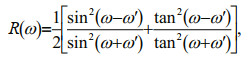 (2)
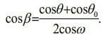
(2)where ω and ωʹ are the incident and refraction angles of sun rays on the inclined surface of the sea, respectively, and the relationship between them is defined as follows:
 (3)
(3) (4)
(4)where θ0 and ϕ0 represent the sun's zenith and azimuthal angles for each pixel, respectively; these parameters can be determined by each pixel's position and imaging time. β denotes the surface tilt angle of a facet on the sea surface (where βN in the 3N image and βB in the 3B image) and is defined as follows:
 (5)
(5)Although Matthews (2005) discussed the geometry of sun glint observations in ASTER images associated with the nadir and back-looking views. However, they only considered one side of the nadir in their calculations, and view angles may differ when ASTER images are obtained from both sides of the nadir. Yang et al. (2015) improved the sun glint geometry model and considered the difference between viewing angles in relation to pixels in multiangle images acquired by the ASTER sensor. These sensor angles can be determined by the scene orientation angle and pointing angle provided in the header file of ASTER images (Yang et al., 2015).
2.4 Extraction of sand-wave crest-linesFrom the results of SSR simulation across a sand crest (He et al., 2015; Yang et al., 2015), the location of a crest line can be identified as the region where the SSR changes abruptly. An investigation of the variations in SSR can show that roughness gradually increases (or decreases) from a sand wave valley to the wave crest, and an abrupt change occurs in a very narrow region near the crest line of sand waves (i.e., the roughness sharply decreases (or increases) first and then gradually increases (or decreases)). With respect to variations in SSR, the variation trend in a very narrow region near the crest line of a sand wave is opposite to that in other regions, and its rate of variation is higher than that in other regions. Therefore, terms "slope-like map" and "aspect-like map" were introduced to describe the variation characteristics of roughness in SSR analysis. The crest line regions of sand waves are considered to be different from those of other regions, and their slope-like values are also higher. For the sand waves in the Taiwan Bank area, the wave directions of the sand waves and the strike of the crest lines are generally close; thus, it can be assumed that the aspect-like values of the sand waves (at a local scale) lie within a certain range of angles, and the extraction of the crest-lines of sand waves can therefore be determined. The specific steps involved in conducting this process in this study are based on the following considerations:
1) Based on an SSR image that contains underwater sand-wave information (Section 2.2), fast Fourier transform (FFT) is conducted to obtain a Fourier spectrum diagram (Fig. 2) from which strong sand-crest information and weak wind stripe information can be determined. The frequency range and distribution angle range of the sand-crest information can be selected from these diagrams. The range of angles shown in Fig. 2 (155°–225°) is the wave direction distribution range of the sand waves. Based on the statistical characteristics of Taiwan Bank sand wave wavelengths, the wavelength range of the underwater sand waves can be determined as lying within a range of 500–1 000 m (Zhang et al., 2014).

|
| Fig.2 FFT spectrum of sea surface roughness in underwater sand-wave regions |
2) The frequency range of the sand-crest information can be selected based on the inverse FFT to filter the SSR results. A comparison of the roughness maps before and after filtering is shown in Fig. 3a–b. The typical cross-sectional lines in Fig. 3g show that the FFT filtering can effectively filter-out interference information, such as wind stripes, and sand-crest information is thus clearer, which is beneficial for use in subsequent analyses.

|
| Fig.3 Sand-wave crest line extraction process and schematic diagrams a. sea surface roughness (SSR) map; b. SSR map after Fourier transform filtering; c. slope-like map; d. aspect-like map; e. two-dimensional histogram of extracted sand-wave crest-lines; f. extracted sand-wave crest-lines; g. cross-sectional profiles of SSR; h. cross-sectional profiles of slope-like and aspect-like maps. The black dash-lines in a–d are the cross-sectional profiles for g and h. |
3) With respect to the methods of calculation used in the terrain analysis, slope and aspect calculations are conducted to obtain the respective slope-like (Fig. 3c) and aspect-like maps (Fig. 3d) based on the filtered SSR information. It is of note that prior to conducting the calculation, the SSR information needs to be normalized to values in the range of 0–1, to ensure a reasonable range of slope-like and aspect-like values.
4) The same typical cross-sectional lines are extracted from the slope-like and aspect-like maps, as shown in Fig. 3h, and the sand-wave direction range is determined as shown in Fig. 2. The regions corresponding to the sand crests are all between 155° and 255°, and significantly higher slope-like values are observed closer to the sand crest. By setting an appropriate threshold, such as 4%, the region in which the slope-like values are greater than 4.0% and where the aspect-like values range between 155° and 255°, defines the crest line region, as shown in Fig. 3e.
5) For the extracted sand-crest regions, the centerline is extracted by a mathematical morphological method, which is the crest line of the sand waves, as shown in Fig. 3f.
2.5 Adaptive partition of subregionsAfter extracting the sand-wave crest-lines, it is necessary to partition the subregions prior to obtaining associated sand-wave crest line information relating to the study area. Underwater sand-wave topography is notable in the study area because topographic changes mainly occur along the wave direction, and there are only small changes in the sand-crest direction. Therefore, sand-wave topography is considered to be a varying one-dimensional topography. The variation trend and extent of sandwave topography in the sand-wave direction are related to the distribution of SSR. The relationship between SSR and sand-wave water depth shows that the SSR undergoes rapid changes at the juxtaposition of the bright and dark stripes of SSR near sand crests, whereas there are only small changes in the SSR near to the wave valleys. By applying equivalent partitioning to SSR, the respective contours are found to be concentrated near to the sand crests but are sparse at locations distant from them. This shows that changes in water depths are significant near to the sand crests but were smaller near their valleys. Such information provides the basis for conducting adaptive partition of the subregions in accordance with the following three considerations:
1) According to the distribution of the crest lines of sand waves, the work area is delineated based on the use of the outer envelope method (Fig. 4a). An auxiliary line is drawn perpendicularly from each of the two endpoints of each crest line related to the sand waves and is extended on both sides to the nearest crest lines or up to the boundary of the work area. The work area is then partitioned into partial areas based on all the crest lines of the sand waves and auxiliary lines (Fig. 4b).

|
| Fig.4 Partition interpolation a and b. the subregion partitioning; c. the water-depth estimation. |
2) Subregion partitioning is applied to each partial area using the Euclidean Distance Equipartition method. First, a specific number of straight lines (auxiliary lines) are uniformly set in a direction perpendicular to the crest lines of the sand waves, and the interval of the auxiliary lines is then set to a value that is approximately equal to five times the interval of the MBES points (r). The location of the center point is calculated according to the intersection of the auxiliary line and the sand-wave crest line, and the center points on all auxiliary lines are then connected to obtain the parting lines of the first partition. Thus, the area between two crest lines of sand waves is partitioned into two subregions. The aforementioned method is used repeatedly to continue partitioning of the two subregions until the width of the subregions is approximately two times the interval of the MBES points.
3) To reduce the number of subsequent calculations and based on the principle that changes in water depth are significant closer to the sand-wave crests but smaller closer to their valleys, the subregions at the sand wave valleys can be merged based on the changes of the SSR in each sand wave subregion. This step can also be skipped to supplement the auxiliary points and to directly estimate the water depth.
2.6 Supplementation of auxiliary points and estimation of water depthsAs supplementary information for the lack of MBES data from a certain number of auxiliary points, the MBES data measured within an interval of 500– 1 000 m are spatially superimposed together with the crest-lines of the sand waves, where the distance between the auxiliary points is the same as the interval between MBES data points (r), and the uniform distribution method is used to determine the location of the auxiliary points. In this respect, the grids covering the work area are established using the interval between MBES data points (r) as the grid size, and the center points of those grids are then used as the locations of the auxiliary points. Auxiliary points are deleted when their distances were less than (r) from the existing MBES data points, and the remaining points are retained as the auxiliary points.
A search range is then set with each auxiliary point as the center point and the spacing of the MBES lines (L) as the radius. The subregion where the auxiliary point is located is determined, and this subregion and all the adjacent subregions are then used as the target area. Accordingly, the MBES data points within the target area are searched, as shown in Fig. 4c. The inverse distance square weighting method (IDSW) is used to determine the water depth values of the auxiliary points, where the water depth values of the searched MBES data points are superimposed on the auxiliary points using the reciprocal of the squared distance as the weighting value. The superposition formula is as follows:
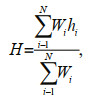 (6)
(6)where H is the estimated water depth of an auxiliary point; Wi=1/di2, where di is the distance from an ith MBES data point to an auxiliary point; and hi is the water depth value of the ith MBES data point.
2.7 Generation of DBM images and accuracy validationAfter estimating the water-depth information for the auxiliary points, the auxiliary points then contain both coordinate information and water-depth information (similar to the measured multibeam water depth points). Therefore, the auxiliary points complemented the water depths of the blank areas between the cross-sections of the MBES lines, and can be combined with the MBES points to map sand-wave topography. Interpolation algorithms, such as IDSW and the Kriging method, can be employed for spatial interpolation to obtain the DBM. To enable the error to be evaluated, the MBES data on the crossed check line are then superimposed onto the DBM according to the spatial location to obtain the corresponding data point pairs of the retrieved water and measured water depths.
3 CASE STUDY 3.1 Study areaThe case study area is the Taiwan Bank, which is located at the southern entrance of the Taiwan Strait (Fig. 5a) between Fujian Province and Taiwan Island; it extends from west to east and its center is located at 23°00′N, 118°30′ E. It is the largest shallow marine sand-wave complex in the world and covers a total area of approximately 16 400 km2 (Zhang et al., 2014). The water depths are relatively shallow, ranging from 10 to 45 m with an average of 20 m. The sand waves are characterized by long wavelengths (500–1 800 m) and tall waves (6–15 m on average), and some have bimodal formations (Boggs, 1974; Cai et al., 1992; Du et al., 2008). Owing to the input of coastal sediments and nonferrous metals, water optical transparency is limited to a maximum of approximately 30 m, but it can be as low as 2–10 m closer to the shore (Li, 2012). Thus, it is difficult for visible light radiation to reach the bottom of the sea in this region. As the flow field evolves, convergence and divergence result from the underwater topography, which affects the SSR. Therefore, sand-wave topography characteristics of the Taiwan Bank were detected using sun glint images.

|
| Fig.5 Case study area location and remote sensing data a. geographic location of the Taiwan Bank; b. location of case study area (pink shading) and check line of multibeam bathymetric data (black line); c. nadir view image; d. back-looking view stereo ASTER image acquired on July 16, 2003 at 02:47:27 UTC. Rectangles highlighted in red are the case study areas that correspond to the pink rectangle in (b). |
Two types of data were used in this case study: a multiangle sun glint remote sensing image dataset, which included ASTER stereo images acquired on 16 July 2003 at 02:47:27 coordinated universal time (UTC) from the central area of the Taiwan Bank (Fig. 5b), and MBES data acquired from May 25 to June 28, 2012.
Figure 5c shows the nadir-looking-view image (NVI) of the 3N channel of the visible and near-infrared (VNIR) sensor in the study area taken on 16 July 2003 at 02:47:27 UTC, and Fig. 5d is the backward-looking-view image (BVI) of the 3B channel of the VNIR sensor obtained 55 s later for the same area. ASTER is an advanced multispectral imager that was installed on the National Aeronautics and Space Administration's (NASA) Terra spacecraft (launched in December 1999), and it captures daily satellite imagery during its orbit of the Earth. The ASTER instrument consists of three separate subsystems: (a) VNIR; (b) shortwave infrared (SWIR); and (c) thermal infrared (TIR). The SWIR and TIR subsystems capture images with a single-angle orientation, while the VNIR subsystem has three bands, a spatial resolution of 15 m, and an additional backward telescope for stereo observations. The 3N channel has the same bandwidth (0.78–0.86 in the near-infrared range) as that of the 3B channel, and it detects the same region 55 s later. The stereo imaging mode was originally designed for terrestrial applications, such as the generation of high-accuracy digital elevation models. However, the high-spatial-resolution (15 m), sensor tilt capability, and backward-looking view from channel 3B give the ASTER imager considerable potential for ocean applications involving multiangle remote sensing.
Most of the sand waves in Fig. 5c are well defined in the high-quality images, and dark and bright stripes are clearly visible. However, the brightness of the entire image increases from west to east, which suggests a matching tendency with sun glint radiance. Relative to the NVI, the brightness of the BVI decreases uniformly over the entire image, as shown in Fig. 5d.
The multibeam bathymetric data were obtained using an R2Sonic 2024 Broadband Multibeam Echo Sounder device with 5th-generation multibeam architecture in 2012. This device can be employed when conducting submarine bathymetry surveys in the range of 1–500 m; it has a frequency range of 200 to 400 kHz, a selectable swath coverage of 10° to 160°, and a beam angle of 0.5°×1° with 256 efficient beams. Our dataset had an adjacent data point spacing equal to 10 m, and there was 500 m between the MBES lines. Given the water depth conditions in the study area, the width of the sounding lines ranged from 100 m to 200 m; therefore, no sounding data were available for an area spanning approximately 300–400 m between the MBES lines. The MBES line ranged from the northeast to the southwest and was approximately perpendicular to the sand waves generated in the study area. In addition, for accuracy validation, we used a single line of MBES data (shown as a black line in Fig. 5b) that obliquely crossed most of the MBES lines. The MBES data had been corrected for tide level.
4 RESULT AND DISCUSSIONThe methods introduced in Section 2 were applied to map and analyze the topography of the Taiwan Bank sand waves using the multiangle sun glint remote sensing images and MBES data. First, an SSR image of the sand-wave area was obtained (sand-wave information of the studied area is clearly shown in Fig. 6a). Based on the information within this image, the final sand-wave bathymetric mapping results were obtained, and Fig. 6b shows the structure and variation characteristics of the sand waves.

|
| Fig.6 Bathymetric mapping results of sand waves within the study area a. sea surface roughness image; b. water depth image. |
A quantitative evaluation of the mapping results was conducted based on the water depth data obtained along the check line. The MBES data consisted of 10 325 points along the check line, which were uniformly selected, and the water depth values were comparatively analyzed with the mapping results of the corresponding points. A scatter plot of these data is shown in Fig. 7a. The two datasets showed good consistency with a correlation coefficient of R2=0.896 2. In addition, the calculated root-mean-square error (RMSE) was 1.77 m, the average water depth at all evaluation points was 35.18 m, and the resulting relative error was 5.03%. The remote sensing-based inversion method of Shao et al. (2014) provides a test accuracy of 4.2 m in the same area; therefore, our method provides obvious accuracy advantages. To analyze the error distribution, a statistical analysis was conducted on the errors of all evaluation points (Fig. 7b). The results showed that the error distribution of the mapping results in the case study area was normally distributed, with the distribution center set at -0.5 m; therefore, most of the errors occurred between -2.0 and 1.0 m. The spatial error distribution was analyzed along the check line as shown in Fig. 7c, where it is evident that the mapped and measured water depths match well in both the crest and valley of most sand waves; however, there are larger errors around the sites at 10 000 m and 13 000 m where the sand wave heights are lower. These results show that the method proposed in this study provides good water depth mapping outcomes for the complex sand waves within a study area measuring 350 km2.

|
| Fig.7 Error analysis of sand-wave water depth mapping results in study area a. scatter plot of error evaluation; b. statistical error distribution diagram; c. error distribution along the check line. |
The results show that, in principle, our proposed method represents a major improvement in the bathymetric mapping of large complex sand waves by incorporating novel methods for extracting crest-lines and a two-stage adaptive partitioning of subregions based on quantitative SSR information. Compared with the manual extraction method proposed by He et al. (2014), our method enables large-scale computer-aided extraction of sand-wave crest-lines and greatly improves the extraction efficiency and accuracy. In addition, compared with experimental studies of simple sand-wave topography with three or four crest-lines (He et al., 2014; Shao et al., 2014), the proposed method uses a two-stage adaptive partitioning method within an area measuring almost 350 km2 that contains many staggered sand waves, and a comparable mapping accuracy is achieved. Calkoen et al. (2001) applied the Alpers and Hennings model-based bathymetry assessment system (BAS) and used SAR images to obtain a water depth sounding accuracy equal to 0.3 m in the sand-wave region of the North Sea in Europe. Although the results obtained here appear unsatisfactory compared to those of their study, the average water depth in our research area is much deeper (30 m compared to 5 m), which means that the relative errors are equivalent. Compared with the BAS method, our method does not require external environmental parameters and it is relatively straight forward to implement. In addition, the water-depth inversions for underwater sand waves proposed by Shao et al. (2014) and Zhang et al. (2015) are only applicable to a small number of sand-wave cross-sections and they cannot meet the water-depth mapping requirements of large-scale complex sand waves. In this respect, the proposed method combines sun glint images with a low accuracy (an RMSE of 4.2 m by Shao et al. in 2014) with highly accurate MBES data (centimeter-level) to achieve relatively good accuracy in a large complex sand wave area.
Although our approach offers advantages over existing remote-sensing-based bathymetry mapping techniques, it also contains certain limitations. One limitation is the distance between multibeam sounding lines. Specifically, a greater distance reduces the number of sounding points used when estimating subregion auxiliary point water depths, which affects the accuracy of the results. For example, He et al. (2014) found that a distance of approximately 1 000 m is acceptable for obtaining good sand wave mapping results within the Taiwan Bank area. Another limiting factor is the wave height of the underwater sand waves. According to the sand-wave remote sensing imaging mechanism, when the wave height of a sand wave is small, the resulting change in SSR is not significant enough to be detected; this affects the accuracy of crest line determinations, which then results in bathymetric mapping errors (Fig. 7c).
5 CONCLUSIONWe proposed a new method based on the use of multiangle sun glint images and sparse MBES data to enable the bathymetric mapping of large, complex sand waves. To validate the effectiveness of this new method, the Taiwan Bank was used as the case study area.
The results show that our method enables the efficient extraction of crest-lines. This is achieved using a quantitative estimation method for SSR data based on the multiangle sun glint remote sensing. The method also involves conducting FFT spectrum analysis, FFT filtering of SSR data, slope-like and aspect-like map analyses and segmentation, and applying a mathematical morphological method to realize the rapid, large-scale extraction of underwater sand-line crest-lines.
In addition, an adaptive subregion partitioning method is implemented. According to the water-depth of the large-scale sand waves and associated mapping, a two-stage subregion partition is adopted, and the corresponding spatial relationship between sand-wave water depths and SSR is considered. Furthermore, the sub-regional auxiliary point estimation method is improved to provide greater continuity in large-scale sand-wave areas, which allows for a more realistic representation of water depth variations.
The results of the case study show that this method enables good bathymetric mapping results to be obtained for large-scale (approximately 350 km2) complex sand-wave areas; in addition, complete topographic data can be successfully obtained from areas even with no MBES data. These results indicate that the proposed method can be used to effectively map large-scale sand-wave topography, and with acceptable mapping errors, even if the acquisition times of the images and data were four years apart. Therefore, it can be employed to reduce the workload associated with MBES, improve efficiency, and reduce costs.
6 DATA AVAILABILITY STATEMENTThe datasets generated and / or analyzed during the current study are not publicly available due to state policy restrictions, but are available from the corresponding author on reasonable request.
7 ACKNOWLEDGMENTThe authors wish to acknowledge the cooperative efforts between NASA and Japan's Ministry of Economy Trade and Industry (METI) during development of the ASTER sensor. The bathymetry datasets used in this study were obtained from the Public Science and Technology Research Fund Project of Ocean (No. 201105001). The authors would like to thank Professor Yan LI from Xiamen University for his comments on this paper.
Allen J R L. 1982. Simple models for the shape and symmetry of tidal sand waves: (1) statically stable equilibrium forms. Marine Geology, 48(1-2): 31-49.
DOI:10.1016/0025-3227(82)90128-1 |
Alpers W, Hennings I. 1984. A theory of the imaging mechanism of underwater bottom topography by real and synthetic aperture radar. Journal of Geophysical Research: Oceans, 89(C6): 10529-10546.
DOI:10.1029/JC089iC06p10529 |
Bao J J, Cai F, Ren J Y, et al. 2014. Morphological characteristics of sand waves in the Middle Taiwan Shoal based on multi-beam data analysis. Acta Geologica Sinica-English Edition, 88(5): 1499-1512.
DOI:10.1111/1755-6724.12314 |
Boggs S Jr. 1974. Sand-wave fields in Taiwan Strait. Geology, 2(5): 251-253.
DOI:10.1130/0091-7613(1974)2<251:SFITS>2.0.CO;2 |
Cai A Z, Zhu X N, Li Y M, Cai Y E. 1992. Sedimentary environment in Taiwan Shoal. Chinese Journal of Oceanology and Limnology, 10(4): 331-339.
DOI:10.1007/BF02843834 |
Calder B R, Mayer L A. 2003. Automatic processing of high-rate, high-density multibeam echosounder data. Geochemistry, Geophysics, Geosystems, 4(6): 1048.
DOI:10.1029/2002GC000486 |
Calkoen C J, Hesselmans G H F M, Wensink G J, et al. 2001. The bathymetry assessment system: efficient depth mapping in shallow seas using radar images. International Journal of Remote Sensing, 22(15): 2973-2998.
DOI:10.1080/01431160116928 |
Cox C, Munk W. 1954. Measurement of the roughness of the sea surface from photographs of the sun's glitter. Journal of the Optical Society of America, 44(11): 838-850.
DOI:10.1364/JOSA.44.000838 |
De Loor G P, Brunsveld van Hulten H W. 1978. Microwave measurements over the North Sea. Boundary-Layer Meteorology, 13(1): 119-131.
DOI:10.1007/BF00913866 |
Du X Q, Li Y, Gao S. 2008. Characteristics of the large-scale sandwaves, tidal flow structure and Bedload transport over the Taiwan Bank in Southern China. Acta Oceanologica Sinica, 30(5): 124-136.
(in Chinese with English abstract) DOI:10.3321/j.issn:0253-4193.2008.05.017 |
He X K, Chen N H, Zhang H G, Fu B, Wang X Z. 2014. Reconstruction of sand wave bathymetry using both satellite imagery and multi-beam bathymetric data: a case study of the Taiwan Banks. International Journal of Remote Sensing, 35(9): 3286-3299.
DOI:10.1080/01431161.2014.902551 |
He X K, Chen N H, Zhang H G, et al. 2015. The brightness reversal of submarine sand waves in "HJ-1A/B" CCD sun glitter images. Acta Oceanologica Sinica, 34(1): 94-99.
DOI:10.1007/s13131-015-0602-2 |
Hennings I, Doerffer R, Alpers W. 1988. Comparison of submarine relief features on a radar satellite image and on a Skylab satellite photograph. International Journal of Remote Sensing, 9(1): 45-67.
DOI:10.1080/01431168808954836 |
Hennings I, Matthews J, Metzner M. 1994. Sun glitter radiance and radar cross-section modulations of the sea bed. Journal of Geophysical Research: Oceans, 99(C8): 16303-16326.
DOI:10.1029/93JC02777 |
Katoh K, Kume H, Kuroki K et al. 1998. The development of sand waves and the maintenance of navigation channels in the Bisanseto Sea. In: Proceedings of the 26th International Conference on Coastal Engineering. American Society of Civil Engineers, Copenhagen. p. 3490-3502, https://doi.org/10.1061/9780784404119.265.
|
Li F. 2012. Annual variations of Secchi depth in the nearshore waters of the western Taiwan Strait during the summers of 1998-2010. Journal of Oceanography in Taiwan Strait, 31(3): 301-306.
|
Li Y, Hu J Y, Li J et al. 2003. Optical image modulation above the submarine bottom topography: a case study on the Taiwan Banks, China. In: Proceedings of the SPIE 4892, Ocean Remote Sensing and Applications. SPIE, Hangzhou, https://doi.org/10.1117/12.466156.
|
Liu Z C, Zhou X H, Chen Y L, et al. 2005. The development in the latest technique of shallow water multi-beam sounding system. Hydrographic Surveying and Charting, 25(6): 67-70.
(in Chinese with English abstract) DOI:10.3969/j.issn.1671-3044.2005.06.020 |
Lyzenga D R. 1977. Reflectance of a flat ocean in the limit of zero water depth. Applied Optics, 16(2): 282-283.
DOI:10.1364/AO.16.000282 |
Lyzenga D R. 1978. Passive remote sensing techniques for mapping water depth and bottom features. Applied Optics, 17(3): 379-383.
DOI:10.1364/AO.17.000379 |
Matthews J P, Yang X D, Shen J, et al. 2008. Structured Sun glitter recorded in an ASTER along-track stereo image of Nam Co Lake (Tibet): an interpretation based on supercritical flow over a lake floor depression. Journal of Geophysical Research: Oceans, 113(C1): C01019.
DOI:10.1029/2007JC004204 |
Matthews J. 2005. Stereo observation of lakes and coastal zones using ASTER imagery. Remote Sensing of Environment, 99(1-2): 16-30.
DOI:10.1016/j.rse.2005.04.029 |
Morelissen R, Hulscher S J M H, Knaapen M A F, et al. 2003. Mathematical modelling of sand wave migration and the interaction with pipelines. Coastal Engineering, 48(3): 197-209.
DOI:10.1016/S0378-3839(03)00028-0 |
Passchier S, Kleinhans M G. 2005. Observations of sand waves, megaripples, and hummocks in the Dutch coastal area and their relation to currents and combined flow conditions. Journal of Geophysical Research: Earth Surface, 110(F4): F04S15.
DOI:10.1029/2004JF000215 |
Shao H, Li Y, Li L. 2011. Sun glitter imaging of submarine sand waves on the Taiwan Banks: determination of the relaxation rate of short waves. Journal of Geophysical Research: Oceans, 116(C6): C06024.
DOI:10.1029/2010JC006798 |
Shao H, Li Y, Li L. 2014. Priori knowledge based a bathymetry assessment method using the sun glitter imagery: a case study of sand waves on the Taiwan Banks. Acta Oceanologica Sinica, 33(1): 120-126.
DOI:10.1007/s13131-014-0375-z |
Whitehouse R, Beech N, Hulscher S J M H et al. 1998. Understanding the behaviour and engineering significance of offshore and coastal sandbanks. In: Proceedings of the 33rd MAFF Conference of River and Coastal Engineers. Keele University, London. p. 2.3.1-2.3.14.
|
Xu J P, Wong F L, Kvitek R, et al. 2008. Sandwave migration in Monterey Submarine Canyon, Central California. Marine Geology, 248(3-4): 193-212.
DOI:10.1016/j.margeo.2007.11.005 |
Yang K, Zhang H G, Fu B, et al. 2015. Observation of submarine sand waves using ASTER stereo sun glitter imagery. International Journal of Remote Sensing, 36(22): 5576-5592.
DOI:10.1080/01431161.2015.1101652 |
Zhang H G, Lou X L, Shi A Q, et al. 2014. Observation of sand waves in the Taiwan Banks using HJ-1A/1B sun glitter imagery. Journal of Applied Remote Sensing, 8(1): 083570.
DOI:10.1117/1.JRS.8.083570 |
Zhang H G, Yang K, Lou X L, et al. 2015. Bathymetric mapping of submarine sand waves using multiangle sun glitter imagery: a case of the Taiwan Banks with ASTER stereo imagery. Journal of Applied Remote Sensing, 9(1): 095988.
DOI:10.1117/1.JRS.9.095988 |
Zhang H G, Yang K, Lou X L, et al. 2018. Observation of sea surface roughness at a pixel scale using multi-angle sun glitter images acquired by the ASTER sensor. Remote Sensing of Environment, 208: 97-108.
DOI:10.1016/j.rse.2018.02.004 |
Zhou J Q, Wu Z Y, Jin X L, et al. 2018. Observations and analysis of giant sand wave fields on the Taiwan Banks, northern South China Sea. Marine Geology, 406: 132-141.
DOI:10.1016/j.margeo.2018.09.015 |