 2022, Vol. 40
Institute of Oceanology, Chinese Academy of Sciences
Article Information
- JIANG Xingjie, ZHANG Tingting, GAO Dalu, WANG Daolong, YANG Yongzeng
- Estimating the evolution of sea state non-Gaussianity based on a phase-resolving model
- Journal of Oceanology and Limnology, 40(5): 1909-1923
- http://dx.doi.org/10.1007/s00343-021-1236-1
Article History
- Received Jun. 10, 2021
- accepted in principle Sep. 26, 2021
- accepted for publication Dec. 4, 2021


2 Laboratory for Regional Oceanography and Numerical Modeling, Pilot National Laboratory for Marine Science and Technology (Qingdao), Qingdao 266237, China;
3 Shandong Key Laboratory of Marine Science and Numerical Modeling, Qingdao 266061, China;
4 Ocean University of China, College of Oceanic and Atmospheric Sciences, Qingdao 266071, China
Rogue, freak, or extreme waves are highly destructive ocean waves that represent serious threats to various marine activities, such as sea voyages, ocean fishing, and oil exploitation. Several physical mechanisms based both on linear and on nonlinear theories have been proposed to explain the formation of such waves (Kharif and Pelinovsky, 2003; Kharif et al., 2009). Comparing to linear theories, it has been suggested that nonlinear mechanisms related to second- and third-order nonlinear wave-wave interactions (Janssen, 2003; Fedele, 2008; Fedele and Tayfun, 2009) can evidently prove the prediction of rogue wave in both aspects of occurrence probability and wave heigh magnitude.
Nonlinear wave-energy focusing caused by such nonlinearities can lead to the formation of rogue waves more frequently and wave surface elevations that generally deviate from the Gaussian (normal) distribution, resulting in non-Gaussian sea states (Longuet-Higgins, 1963). Commonly used measures of the non-Gaussianity of sea state are skewness μ3 and (excess) kurtosis μ4:
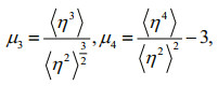 (1)
(1)where η denotes the wave surface elevation, and the terms in angled brackets denote statistical averages. With the consideration of nonlinearities up to third-order, it is clear that, skewness is contributed entirely by second-order nonlinear interactions involving bound waves (Tayfun, 1980; Tayfun and Fedele, 2007; Fedele and Tayfun, 2009; Janssen, 2009), and that kurtosis includes a dynamic component (μ4free) attributable to third-order quasi-resonant interactions (Janssen, 2003; Mori and Janssen, 2006) between free waves and another bound component (μ4bound) induced by both second- and third-order bound-wave nonlinearities (Tayfun, 1980; Tayfun and Lo, 1990; Fedele, 2008; Fedele and Tayfun, 2009; Janssen, 2009); these variables can be expressed as follows:
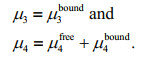 (2)
(2)The non-Gaussianity of sea state is also sensitive to the geometries of the corresponding wave spectrum, and this relation has been well established using theoretical models (e.g., Janssen, 2003, 2009; Fedele and Tayfun, 2009) and confirmed by laboratory and numerical experiments (e.g., Onorato et al., 2009a, b; Toffoli et al., 2009; Waseda et al., 2009; Fedele, 2015). Generally, at least three geometric factors—wave steepness (hereafter, SP), bandwidth (BW), and directional spreading (DS)—can influence skewness, kurtosis, or both. For steeper SP and narrower BW and DS, it can be concluded that the deviation from Gaussianity will be greater, resulting in higher probability of rogue wave occurrence in such a sea state.
Following the above investigations, it has been established that two types of approach can be used to estimate skewness and kurtosis using the three spectral geometric factors. One is based on formulae/equations derived from theoretical wave models such as the Zakharov equation (Zakharov, 1968; Janssen, 2003) and the Tayfun-Lo model (Tayfun and Lo, 1990); and the other is based on phase-resolving models such as the high-order spectral method (HOSM) (Dommermuth and Yue, 1987; West et al., 1987) and the modified nonlinear Schrödinger equations (MNLS) (Dysthe, 1979; Trulsen and Dysthe, 1996).
Estimation of non-Gaussianity based on theoretical formulae and equations is highly convenient, and such estimates can certainly be applied to assess the non-Gaussianity associated with the evolution of sea state. Some methods have even been adopted in operational rogue wave forecasting systems, such as the ECMWF-IFS WAM (Janssen and Bidlot, 2009; ECMWF, 2016; Janssen, 2018) and the Space-Time Extremes (STE) forecasting system included in version 5.16 of WWⅢ (Barbariol et al., 2015; The WAVEWATCH Ⅲ Development Group, 2016; Barbariol et al., 2017). However, the indicators of skewness and kurtosis obtained using theoretical models, must first be obtained from theoretical models derived under the narrowband assumption in an environment with unidirectional wave propagation. When applying these indicators in scenarios with real sea conditions, specific parameters representing the spectral geometry are selected and undetermined parameters are introduced. Moreover, for the indicators adopted in rogue wave forecasting systems, calibrations are performed according to the final forecasting results; therefore, estimation of the indicators must balance the consideration of the spectral geometric factors and the other factors. Details regarding the process of calibrating operational non-Gaussianity indicators can be found in Barbariol et al.(2015, 2017) for the WWⅢ-STE system and in ECMWF Technical Memoranda (Janssen and Bidlot, 2009; Janssen, 2018) for the ECMWF-IFS system; the latter can also be found in the Appendix of this paper.
In comparison with theoretical models, phase-resolving models can be used to assess arbitrary two-dimensional (2D) spectra without any spectral shape limitations. These models adopt a given 2D spectrum as the initial wave field and simulate the evolution of surface elevations within a designed duration. Then, according to Eq.1, the corresponding skewness and kurtosis can be obtained based on the statistics of the surface elevations in the simulated wave field. The accuracy and feasibility of such models have been well verified by laboratory experiments (e.g., Toffoli et al., 2010). However, phase-resolving simulations are cumbersome, and performing such simulations based on wave spectrum time series obtained during sea state evolution is very time consuming. Therefore, the "phase-resolved" non-Gaussianity with the evolution of the sea state of interested can hardly be obtained and analyzed.
This paper presents a new approach that makes estimation of the phase-resolved non-Gaussianity more convenient. Using the estimation approach, phase-resolved non-Gaussianity can now be illustrated throughout the evolution of sea states of interest, not just at a few specific times. The remainder of this paper is organized as follows. The establishment of the estimation approach is introduced in Section 2. The application and validation of the approach based on certain sea states with rogue waves are described in Section 3. Finally, a discussion and the derived conclusions are presented in Sections 4 and 5, respectively.
2 ESTABLISHMENT OF THE ESTIMATION APPROACH 2.1 Experimental environment based on the HOSMThe HOSM numerical algorithm (Dommermuth and Yue, 1987; West et al., 1987) is dedicated to solve the Laplace equation for the velocity potential ϕ:
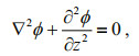 (3)
(3)in a fluid, which is assuming to be inviscid and incompressible and the flow is irrotational. And surface elevations η can be obtained by solving Eq.3 at surface level z=η using the following equations:
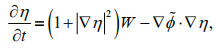 (4)
(4) (5)
(5)where 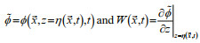
In this study, the HOSM experimental environment was established based on the open-source software package HOS-ocean ver. 1.5 (Ducrozet et al., 2016), which was developed at the Laboratoire de recherche en Hydrodynamique, Énergétique et Environnement Atmosphérique of the École Centrale de Nantes (France). HOS-ocean has been extensively validated in terms of nonlinear regular wave propagation (Bonnefoy et al., 2010), and it has also been widely adopted in previous research for modeling rogue wave sea state (e.g., Ducrozet et al., 2007; Ducrozet and Gouin, 2017; Jiang et al., 2019). HOS-Ocean can ensure the stability and convergence of the calculations. For example, all aliasing errors generated in the nonlinear terms can be removed. Time integration is performed with an efficient fourth-order Runge-Kutta Cash-Karp scheme, and the time step can be automatically selected to achieve a desired level of accuracy (or "tolerance", with typical values in the range of 10-7–10-5; in this study, the accuracy achieved was 10-7). Moreover, a relaxation period of 10Tp (where Tp denotes the peak wave period) is often considered (as was the case in this study) to remove numerical instabilities attributable to fully nonlinear computations that start with linear initial conditions (Dommermuth, 2000). Additional details can be found in Ducrozet et al.(2016, 2017) and Ducrozet and Gouin (2017).
The HOSM experimental environment established in this study considers a physical space of size Lx=xlen×λp and Ly=ylen×λp, where xlen=ylen=25.5, λp is the wavelength at the peak frequency, and the discretization of the space is set as Nx×Ny=256×256. The HOSM is a pseudospectral method which means certain operators including the nonlinear terms are treated in the physical space instead of the spectral space, and the transforms between the physical and spectral spaces are handled efficiently using fast Fourier transforms. Thus, the spectral resolution of the pseudospectra can be determined as Δkx, y=2π/Lx, y, and the spectral space extends from zero to kmax=(Nx, y–1)/2×Δkx, y, where kmax is the cutoff frequency. Additionally, the HOSM cannot deal with wave breaking issues; therefore, a typical cutoff frequency of kmax=5kp is generally adopted in simulations to obtain accurate solutions for the most energetic parts of the spectrum and to restrict the breaking of waves in the wave field to a very limited range (Ducrozet et al., 2017). For both the physical and the spectral spaces, the x-direction is taken as the principal direction of the pseudospectra, the y-direction is horizontal and perpendicular to the x-direction, and the z-direction in the physical space points vertically down with a consideration of infinite water depth.
The effects of spectral geometries on non-Gaussianity can be associated only with nonlinear wave-wave interactions, and therefore the HOSM simulations in this study considered only the wave-wave nonlinearities and ignored other factors that might influence the non-Gaussianity of the simulated wave fields, that is, wind force and energy dissipation due to breaking. According to current research, the non-Gaussianity of the sea state is mainly related to second- and third-order nonlinearities, nonlinearities up to the third order (i.e., M=3) were considered in the simulations.
2.2 Initial conditionTo ensure that the initial conditions of the HOSM simulations were close to those of real sea states, the Joint North Sea Wave Project (JONSWAP) spectrum and specific directional spreading were introduced. The JONSWAP spectrum (Hasselmann et al., 1973; Goda, 1988, 1999) can be expressed as follows:
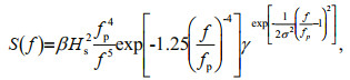 (6)
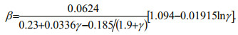
(6)where Hs (m) is the significant wave height and fp (Hz) is the peak frequency, which is also the reciprocal of the peak period Tp. Parameter σ=0.07 when f≤fp and σ=0.09 when f > fp. Parameter γ is the peak enhancement factor, which is related to the BW of Eq.6. Parameter β in Eq.6 can also be expressed in terms of γ as follows:
 (7)
(7)The adopted DS relations (Socquet-Juglard et al., 2005) were as follows:
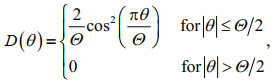 (8)
(8)where the spreading parameter Θ in degrees (°) or radians (rad) indicates that energy is distributed within the range of Θ/2 on both sides of the principal direction (0° or 0 rad). Finally, the 2D initial spectra in the HOS simulations are generated as follows:
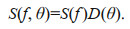 (9)
(9)The three spectral geometric factors in Eqs.6 & 8 are adjustable, and various initial conditions can be generated by considering different combinations of these factors. Based on Eq.6, the expression for SP is as follows:
 (10)
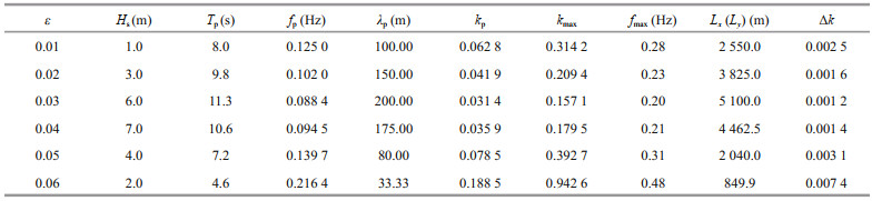
(10)where Hs is the significant wave height and λp is the wavelength at the peak frequency, which can be calculated from fp according to the linear dispersion relation. Thus, SP is determined based on both Hs and fp(Tp) in Eq.6. According to observations in the northern North Sea (deep water) from 1973 to 2001 (Haver, 2002), ε is generally < 0.06 and most frequently in the range of 0.01–0.02 (Fig. 1). To cover all observed sea conditions, the value of ε for the initial spectra was set to vary within the range of 0.01–0.06, and considering the number of calculations involved in the simulations, the interval was set to 0.01. Furthermore, without loss of generality, each value of ε in the range was associated with a unique combination of Hs and Tp. The settings of SP, together with the corresponding simulated physical and pseudospectral spaces, which are closely related to λp(Tp), are listed in Table 1.

|
| Fig.1 Combined Hs-Tp distribution observed in the northern North Sea from 1973 to 2001 Reprinted with permission (Ducrozet et al. 2017), Copyright 2017, Elsevier, in which only the line of ε=0.06 is the original data and the lines of ε=0.01-0.05 are from this study. |
|
The BW and DS values of the initial spectra can be determined from γ and Θ, respectively. For BW, parameter γ was set to vary within the range of 1.0–7.0 in accordance with the JONSWAP observations at an interval of 1.0. For DS, the range of the spreading parameter Θ was set to 8°–340°, and the interval of Θ in the range of 8°–176° (180°–340°) was set at 8° (20°).
Finally, the total number of initial spectra with adjustable ε, γ, and Θ values was 6×7×31=1 302, and the HOSM simulations were performed for each individual case. Regardless of how the combination of Hs and Tp might vary, the number of waves involved in each initial wave field will always be 25.5×25.5 (Section 2.1).
2.3 Skewness and kurtosis indicatorsOne complete HOSM simulation with a given initial spectrum is called one realization. Notably, previous experiments revealed that, with the nonlinearities that are up to third order, the most significant variations in skewness and kurtosis in the simulated wave fields all occurred in the first 180Tp of the simulation duration, and subsequent changes in both skewness and kurtosis were minimal because the simulated wave field tended to be Gaussian. Thus, the simulation duration of each realization was set to 180Tp. The skewness μ3 and kurtosis μ4 were calculated using Eq.1 based on the 256×256 surface elevations for each of the output simulated wave fields, and the output interval was 1Tp. Notably, the temporal evolutions of μ3 and μ4 obtained from one realization were random and unstable, and that obtaining averages of them from a number of realizations with the same initial spectrum would significantly reduce uncertainty, see Section 2.4.
We considered the indicators μ3 and μ4, which can represent the average characterization of nonGaussianity during each 180Tp simulation. Therefore, the temporal evolutions of μ3 and μ4 were first averaged for the final 170Tp (denoted 


 (11)
(11)which could be used as non-Gaussianity indicators to identify the temporal evolution of skewness and kurtosis. Thus, the non-Gaussianity of the simulated wave fields corresponding to the initial spectra with certain combinations of ε, γ, and Θ was comparable.
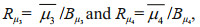
2.4 Number of repetitionsIncorporation of a large number of repetitions in an averaging process generally produces results that are stable and convergent. Therefore, eight convergence tests were performed to determine the minimum number of repetitions to be averaged. Each test involved an individual initial condition, as listed in the right part of Fig. 2. For each initial condition, 100 realizations were conducted, of which n were then selected at random to produce a collection named Cn. For n=30, 40, 50, …, 100, there were eight collections to establish. The indicators Rμ3 and Rμ4 for each collection are shown in Fig. 2.

|
| Fig.2 Results of convergence tests for the number of repetitions included in the averaging process a. test results for Rμ3; b. test results for Rμ4. |
It can be seen from Fig. 2 that satisfactory convergence could be achieved for both Rμ3 and Rμ4 after 60–70 realizations. Accordingly, the number of repetitions involved in the averaging procedure was set to 80.
2.5 Spectral geometries and non-Gaussianity indicatorsThe obtained non-Gaussianity indicators constituted two reference sets for skewness and kurtosis, here denoted Rμ3 (ε, γ, Θ) and Rμ4 (ε, γ, Θ), respectively. Parts of the two references are illustrated in Fig. 3. As shown in Fig. 3a–d, the overall trends of Rμ3 and Rμ4 are affected by ε, γ, and Θ, confirming that as the value of ε increased, the value of γ increased, or as the value of Θ decreased, the value of Rμ3 and Rμ4 increased. Moreover, the values of Rμ3 and Rμ4 change continuously with the three geometric parameters. As illustrated in Fig. 3a–b, Rμ3 is affected most evidently by the SP parameter ε; moreover, Θ tends to cause slight increase in Rμ3 as it approaches 0°, as shown in the upper-left corner of Fig. 3a. Additionally, γ can influence Rμ3 when Θ is narrow, as shown in the upper-left corner of Fig. 3b. In Fig. 3c–d, within the range where Θ is extremely narrow (e.g., Θ≤20°), Rμ4 decreases markedly as Θ widens; when Θ is beyond the extremely narrow range, the value of Rμ4 decreases, but this decrease is much slower than that when Θ widens within the extremely narrow range. Parameters γ and ε can also have certain effects on Rμ4. For example, larger values of γ and ε result in larger values of Rμ4, and the corresponding increase becomes significant when Θ is extremely narrow. Same results can be found in the previous research (Gramstad and Trulsen, 2007), but in which the spectral geometries that can influence kurtosis were discussed in the form of spectral width in the direction of the main wave propagation (or alternatively the Benjamin-Feir Index) and in the direction perpendicular to the main wave propagation (or alternatively the crest length).

|
| Fig.3 Parts of the non-Gaussianity references for Rμ3 with γ=3.0 (a) and ε=0.02 (b), and for Rμ4 with γ=3.0 (c) and ε=0.02 (d) The colors denote the magnitude of the values of the two references (larger values are indicated by yellow and lower values are indicated by blue). |
It should be noted that Rμ could be negative for some combinations of (ε, γ, Θ) owing to two possible factors. First, some of the simulated kurtosis values were rather small, and they oscillated slightly and randomly near 0, resulting in a negative average value. Second, μ4free might be influenced by defocusing of wave energy as the ratio of BW to DS increases (Fedele, 2015). Therefore, negative Rμ4 values represent sea states with inactive MI or the defocusing of energy, both factors might lead to decreased possibility of rogue waves forming in such sea states.
2.6 Development of the extraction approachAs Rμ3 and Rμ4 change continuously with ε, γ, and Θ, the non-Gaussianity indicators can be obtained via three-dimensional interpolation using an arbitrary combination of (εi, γi, Θi), where subscript i indicates an arbitrary position in each of the ranges of ε, γ, and Θ, respectively. The crucial step is to determine how the parameters εi, γi, and Θi that appear in the non-Gaussianity references might be related to the geometries of SP, BW, and DS in a given spectrum.
The SP for any spectrum can be calculated as follows:
 (12)
(12)where 
For DS, the spreading parameter σθ (Kuik et al., 1988) can be adopted as follows:
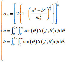 (13)
(13)By applying Eqs.8–13, we find that σθ increases monotonically with Θ within the range of Θ∈[8°, 340°], as indicated by the black solid line in Fig. 4a. This line can be fitted by a second-order polynomial, shown as the red dashed line in Fig. 4a, and expressed as follows:
 (14)
(14)

|
| Fig.4 Polynomials fitted for σθ(Θ) (a) and Qp(γ) (b) |
After σθ has been calculated from the given spectrum, it is easy to solve for the root of Eq.14 in the range of 8°–340° to obtain the corresponding Θi.
For BW, the parameter Qp (Goda, 1970) can be used:
 (15)
(15)Similarly, applying Eqs.6–15 reveals that Qp increases monotonically with γ in the range of γ∈[1, 7], as indicated by the black solid line in Fig. 4b. This line can also be fitted by a second-order polynomial, shown as the red dashed line in Fig. 4b, and expressed as follows:
 (16)
(16)Thus, parameter γi can be obtained by solving for the root of Eq.16 in the range of (γ∈[1, 7]) with Qp calculated from the given spectrum.
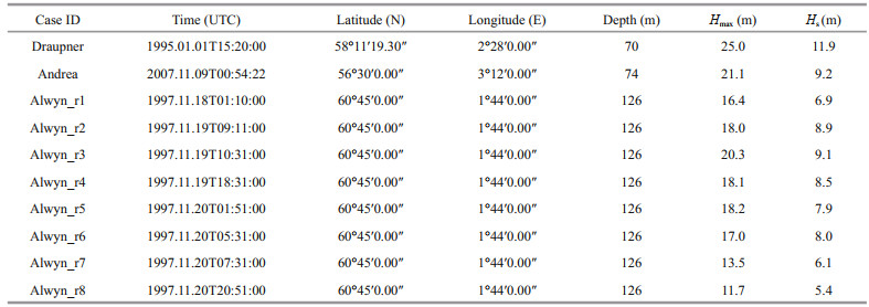
3 APPLICATION AND VALIDATION OF THE ESTIMATION APPROACH 3.1 Rogue wave events and wave modelingThe newly established approach is applied to some sea states with occurrence of rogue waves. The 10 rogue wave events discussed in this section were all observed using laser sensors installed on oil platforms in the North Sea. The locations of the platforms and UTC times at which the events occurred are listed in Table 2, together with the synchronously observed maximum wave heights (Hmax) and significant wave heights (Hs), which were digitized from Magnusson and Donelan (2013) for Draupner and Andrea and from Guedes Soares et al. (2003) for the Alwyn events.
In this study, the wave fields containing the selected events were reproduced using the WWⅢ wave model ver.5.16 (The WAVEWATCH Ⅲ Development Group, 2016). The modeled spectral space was set with 36 directions at intervals of 10° and 35 frequencies spaced from 0.042 to 1.05 Hz as a geometric progression with a ratio of 1.1. The computational grids of the physical area modeled, as illustrated in Fig. 5, include an outer grid named NS4 (50°N–78°N, -18°E–15°E) with 0.25°×0.25° resolution and an inner grid named NS8 (52°N–68°N, -6°E–7°E) with 0.125°×0.125° resolution. Bathymetric data were obtained from ETOPO1 of the National Oceanic and Atmospheric Administration (NOAA) National Geophysical Data Center (NGDC) (National Centers for Environmental Information, 2017), and the wind force adopted in the simulations were derived from ECMWF-ERA5 reanalysis hourly data (Copernicus, 2018). As indicated by the Case IDs listed in Table 2, the modeling started 30 days before and ended 1 day after the occurrence of the Draupner and Andrea events, while for the Alwyn events, the modeling commenced 30 days before Alwyn_r1 and concluded 1 day after Alwyn_r8.

|
| Fig.5 Computational grids of the North Sea |
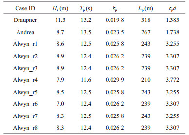
Some of the simulated bulk wave parameters are illustrated in Fig. 6a–d together with observed data digitized from published research for comparison. Comparison of the black solid lines denoting the digitized observations with the blue lines of the simulations reveals acceptable reproduction of the observed sea states; thus, these data provide a reliable foundation for the following analyses. The simulated significant wave height Hs, peak wave period Tp, peak wavenumber kp, peak wavelength Lp, and parameter kpd (kp×d, where d is the water depth at the sites; Table 2) at the times of occurrence of all the rogue wave events are listed in Table 3.

|
| Fig.6 Comparison of simulated results and observations for the Draupner (a), Andrea (b), and Alwyn (c)–(d) events The blue lines depict simulated results, and the black lines (asterisk) depict the digitized observations from Table 1 and Fig. 3 of Magnusson and Donelan (2013) for (a) and (b) and from Table 1 of Guedes Soares et al. (2003) for (c) and (d). The vertical dashed lines denote the times of rogue wave occurrence. |
To validate the estimation approach, additional HOSM simulations were performed based on the same experimental environment as that established in Section 2.1. However, the initial conditions were replaced with modeled wave spectra for the 10 events, and simulations that considered the second-order nonlinearities (M=2) only and both the second- and third-order nonlinearities (M=3) were performed separately to elucidate the dominant mode in the wave fields. A similar approach was used in previous research (Fedele et al., 2016) in which the Draupner and Andrea events were studied.
The results of the additional simulations are illustrated in Fig. 7 and listed in Table 4. As shown in the upper-right corner of Fig. 7, each panel titled with a Case ID contains upper and lower parts exhibiting the temporal evolutions of skewness μ3 and kurtosis μ4 of the simulated wave field, respectively, and the x-axis in each panel represents the time duration with a dimensionless form of time (Tp). The blue and red lines shown in both parts of each panel depict the μ3 and μ4 simulated when considering M=2 and M=3, respectively. The corresponding non-Gaussian indicators (here, denoted Rμ3rw and Rμ4rw) obtained via the newly proposed estimation approach are presented by the black solid lines, and for comparison with the simulated blue and red lines, these two indicators have been multiplied by the benchmarks of Bμ3 and Bμ4, respectively (i.e., black lines in both parts of each panel represent the values of Rμ3rw×Bμ3 and Rμ4rw×Bμ4). For each event identified by a Case ID in Table 4, the non-Gaussianity indicators (Rμ3rw×Bμ3, Rμ4rw×Bμ4), mean values of μ3 and μ4 for M=2 and M=3 (


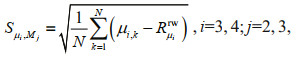 (17)
(17)

|
| Fig.7 Results of the additional HOSM simulations Each panel titled with a Case ID contains upper and lower parts exhibiting the temporal evolutions of μ3 and μ4 of the simulated wave field, respectively; and the x-axis in each panel represents the time duration with a dimensionless form of time (Tp). The blue and red lines shown in both parts of each panel depict μ3 and μ4 simulated when considering M=2 and M=3, respectively; and the black lines denote the Rμ3rw ×Bμ3 and Rμ4rw ×Bμ4 indicators obtained via the estimation approach, respectively. |
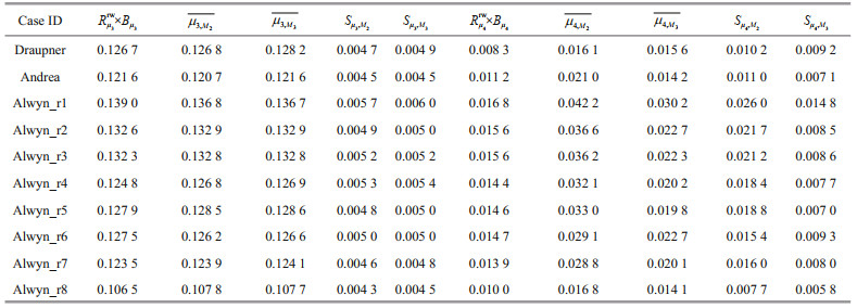
where N=170 denotes the number of μ3 or μ4 samples in the final 170Tp of each of the HOSM simulations (see Section 2.3).
As shown in the upper part of each panel in Fig. 7, the Rμ3rw (×Bμ3) indicator agrees well with the skewness obtained from the simulated wave fields for both M=2 and M=3 nonlinearities, and in the lower part, as expected, Rμ3rw(×Bμ3) is best matched to the kurtosis obtained from the simulated wave fields for M=3. Table 4 also shows that the values of Rμ3rw×Bμ3, 


Throughout the evolution of the simulated sea states, the indicators Rμ3rw and Rμ4rw estimated via the newly proposed approach are shown in Fig. 8, and the indicators for the Draupner (Fig. 8a and d), Andrea (Fig. 8b & e), and Alwyn (Fig. 8c & f) events are depicted by the magenta, blue, and red solid lines, respectively. In each panel of Fig. 8, the vertical dashed lines denote the times of rogue wave occurrence, and the horizontal lines represent (from top to bottom) the 90%, 75%, 50%, 25%, and 10% quantiles of each indicator (for Rμ3rw the values are 0.485 5, 0.439 3, 0.362 5, 0.218 1, and 0.148 4, and for Rμ4rw the values are 0.037 5, 0, 030 7, 0.021 9, 0.007 6, and 0.003 8) obtained within all the modeled durations at the three locations (about three months). The quantiles can help determine the level of the parameter and indicator in the evolution of sea state, and it is noted that the quantiles of the phase-resolved non-Gaussianity indicators now can be obtained because of the application of the newly proposed approach. The values of each indicator at the times of event occurrence are listed in Table 5.

|
| Fig.8 Non-Gaussianity indicator variations during the rogue wave events The indicators for the Draupner (a and d), Andrea (b and e), and Alwyn (c and f) events are depicted by the magenta, blue, and red solid lines, respectively. In each panel, the vertical dashed lines denote the times of rogue wave occurrence, and the horizontal lines represent (from top to bottom) the 90%, 75%, 50%, 25%, and 10% quantiles of each indicator obtained within all the modeled durations at the three locations. |
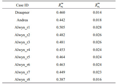
As shown in Fig. 8a–c, the Rμ3rw values at the times of event occurrence are reasonably similar and greater than the 75% quantiles (even over 90% at times during the Alwyn events), and such a situation can persist for several to dozens of hours both before and after event occurrence. For Rμ4rw, Fig. 8d–f reveals that the kurtosis of the sea state does not exhibit any abnormality in comparison with that at the other times simulated, and the values of Rμ4rw for the Draupner and Andrea events are even lower than the 50% quantile.
Thus, it can be concluded that the selected rogue wave events all occurred in non-Gaussian sea states with relatively large skewness, but normal kurtosis. Finally, it should be noted that high values of both Rμ3rw and Rμ4rw according to the quantiles could be found at times before the occurrence of the selected events, suggesting that the probability of rogue wave generation in such sea states was high. However, large values of Rμ3rw and Rμ4rw just indicate higher probability, rather than evidence of rogue wave occurrence; and on the other hand, rogue waves might have been generated in those sea states, but have not been observed.
4 DISCUSSIONTo assess the differences in non-Gaussianity indicators estimated using theoretical formulas and the newly proposed approach, several operational indicators adopted in the extreme wave forecasting system of the Integrated Forecasting System operated by European Centre for Medium-Range Weather Forecasts (ECMWF-IFS) are adopted here as an example. The meaning of each indicator and the methods used for calculating them are given in the Appendix. The evolution trends of the operational indicators are illustrated in Fig. 9, where the colored, horizontal, and vertical lines depict the same events, quantiles, and times just the same as Fig. 8.

|
| Fig.9 Non-Gaussianity indicators obtained by the operational rogue wave forecasting system (ECMWF-IFS) The indicators for the Draupner (a, d, g, and j), Andrea (b, e, h, and k), and Alwyn (c, f, i, and l) events are depicted by the magenta, blue, and red solid lines, respectively. In each panel, the vertical dashed lines denote the times of rogue wave occurrence, and the horizontal lines represent (from top to bottom) the 90%, 75%, 50%, 25%, and 10% quantiles of each indicator obtained within all the modeled durations at the three locations. |
Figure 9a–c shows that indicator C3, representing skewness, exhibits higher values (greater than the 75% quantile) at the time of event occurrence than at other times; moreover, such a situation also persist for several to dozens of hours around the occurrence of the events, just confirming the Rμ3rw results in Fig. 8. However, different from the normal values of kurtosis indicator Rμ4rw found at the times of rogue wave occurrence, the kurtosis indicator C4 (Fig. 9d–f) displays abnormal behavior (even greater that the 90% quantile) in comparison with that of the kurtosis obtained at other moments. Furthermore, as can be observed in the lower panels of Fig. 9, indicators C4bound (Fig. 9g–i) and C4free (Fig. 9j–l), which are associated with the bound and free parts of kurtosis, respectively, both exhibit extremely high values at the times of event occurrence; nevertheless, the contribution of C4free to parameter C4 was much smaller than the contribution of C4bound, and the abnormality of C4 at the times of rogue event occurrence was mainly influenced by C4bound.
As expressed in Eqs.2 & A2 (from Appendix), kurtosis comprises both a dynamic (free) part and a bound part. The dynamic contribution is relatively small; for example, it can be < 10% of the bound component in a normal sea state with broad BW and DS (Annenkov and Shrira, 2014); however, it can reach high levels in specific wave environments, suggesting that MI are active (Janssen, 2003; Fedele, 2015). The C4free at the occurrences of the events are found being > 20% of the C4bound, which is slightly larger than a "normal" value expected. However, the lack of notable discrepancies between the black (M=2) and red (M=3) lines in the lower part of each panel of Fig. 7 indicates that the kurtosis of the selected rogue wave sea states is dominated by second-order nonlinearities, thus, the third-order nonlinearities and the associated MI are inactive; similar conclusions can also be found in Fedele et al. (2016). As mentioned previously, the operational indicators derived from the theoretical formulae might not be suitable for real sea states, thus, the prominent C4 values found at the times of rogue wave occurrences might be caused by an improper calibration. It should be noted that the estimation results obtained with the phase-resolving model, including the Rμ3 and Rμ4 values obtained in this study, might also be incomplete. It is difficult to discuss which kind of estimation is correct or not with the current results, and that is not the main purpose of this study.
The non-Gaussianity indicators obtained in different ways can provide different perspectives for studying rogue wave sea states. And it is not the first time that a phase-resolving model, such as HOSM, has been applied to assess rogue sea states (e.g., Trulsen et al., 2015; Fedele et al., 2016; Jiang et al., 2019). However, phase-resolving simulations can be performed only using several spectra selected from the full spectral evolution of the sea state because full simulations can be cumbersome. In this study, using the precalculated dataset and the extraction approach, phase-resolved non-Gaussianity indicators can be obtained conveniently. Thus, the "normal" or "abnormal" behaviors of sea state non-Gaussianity can be identified according to the statistics of the phase-resolved indicators, which are derived throughout the simulated sea states. Therefore, this study provides a new perspective for studying non-Gaussian sea states and the associated rogue wave sea states, and such studies can be performed based on the phase-resolved non-Gaussianity throughout the evolution of sea states of interest, not just at a few specific times.
With respect to real ocean conditions, our model is certainly an oversimplification; for example, it focuses purely on the nonlinearities among waves, ignoring other physical mechanisms that might influence non-Gaussianity, e.g., wind forcing, wave breaking. Furthermore, the interaction between two wave systems were also ignored, regarding that for two systems do not interact much, the combined wave system appears to be more Gaussian than the corresponding partitioned wave systems (Støle-Hentschel et al., 2020). Therefore, the model was established based only on unimodal spectral shapes and bimodal shapes were ignored. And in the application, the quantiles are just obtained based on samples simulated in a few months, involving more samples might provide more suitable criterion. Further improvement of the new estimation approach can be done in future studies.
5 CONCLUSIONIn this study, we established a systematic approach for estimating the evolution of sea state non-Gaussianity. The newly established approach includes: i) a set of precalculated indicators representing the relation between sea state non-Gaussianity and various combinations of the SP, BW, and DS geometries, and ii) an approach that can extract the skewness and kurtosis indicators from the precalculated dataset for given 2D spectra. Because the precalculated dataset was obtained based on HOSM (phase-resolving) simulations, the indicators can be applied to real sea states without calibration of spectral shapes. With the newly developed extraction approach, estimating the phase-resolved non-Gaussianity of a given sea state becomes convenient, and the phase-resolved non-Gaussianity can be estimated with the evolution of sea state. Validation of the estimation approach was performed based on analysis of sea states in which real rogue waves occurred. The sea states were reproduced using the spectral wave model WWⅢ, and additional HOSM simulations were conducted with simulated wave spectra at the time of occurrence of the rogue wave events. The acceptable goodness of fit of the extracted indicators to the simulated results verified the feasibility of the estimation approach for use in real wave environments.
With the estimation approach, the evolution of the phase-resolved non-Gaussianity in the selected sea states was illustrated. It is found that the selected rogue wave events all occurred in non-Gaussian sea states with relatively large skewness, but normal kurtosis; and that large values of both the skewness and kurtosis indicators can be found at times before the occurrence of the selected events, suggesting high probability of rogue wave generation in such sea states. And it should be noted that the "large" and "normal" judgements given above are based on the statistics of the phase-resolved non-Gaussiniaty indicators, which are obtained throughout the evolution of the simulated sea state.
In comparison with the evolution trends of certain operational indicators derived from theoretical formulae, different behaviors of non-Gaussianity of the same selected the sea states are found. Although, the results of the newly proposed approach seem more reasonable, it is difficult to discuss which kind of estimation is better; and the newly proposed approach still has defects. However, this study provides a new perspective for studying the non-Gaussian rogue wave sea states, and further research could be performed on this basis.
6 DATA AVAILABILITY STATEMENTThe data that support the findings of this study are available on request from the first author Xingjie JIANG (jiangxj@fio.org.cn) or the corresponding author Tingting ZHANG (zhangtt@fio.org.cn).
7 ACKNOWLEDGMENTWe thank Guillaume Ducrozet and Yves Perignon from the Research Laboratory in Hydrodynamics, Energetics and Atmospheric Environment (LHEEA) of the École Centrale de Nantes and The French National Centre for Scientific Research (CNRS) for their assistance in helping us understand the HOSM method and the use of HOS-ocean.
Electronic supplementary material
Supplementary material (Appendix) is available in the online version of this article at https://doi.org/10.1007/s00343-021-1236-1.
Annenkov S Y, Shrira V I. 2014. Evaluation of skewness and kurtosis of wind waves parameterized by JONSWAP spectra. Journal of Physical Oceanography, 44(6): 1582-1594.
DOI:10.1175/JPO-D-13-0218.1 |
Barbariol F, Alves J H G M, Benetazzo A, Bergamasco F, Bertotti L, Carniel S, Cavaleri L, Chao Y Y, Chawla A, Ricchi A, Sclavo M, Tolman H. 2017. Numerical modeling of space-time wave extremes using WAVEWATCH Ⅲ. Ocean Dynamics, 67(3): 535-549.
DOI:10.1007/s10236-016-1025-0 |
Barbariol F, Alves J H G M, Benetazzo A, Bergamasco F, Bertotti L, Carniel S, Cavaleri L, Chao Y Y, Chawla A, Ricchi A, Sclavo M, Tolman H. 2015. Space-time wave extremes in WAVEWATCH Ⅲ: implementation and validation for the Adriatic Sea case study. In: Proceedings of the 14th International Workshop on Wave Hindcasting and Forecasting. Key West, Florida. http://www.waveworkshop.org/14thWaves/index.htm. Access on 2022-04-25.
|
Bonnefoy F, Ducrozet G, Le Touzé D, Ferrant P. 2010. Time domain simulation of nonlinear water waves using spectral methods. In: Ma Q W ed. Advances in Numerical Simulation of Nonlinear Water Waves. World Scientific, Hackensack. p. 129-164, https://doi.org/10.1142/9789812836502_0004.
|
Copernicus. 2018. ERA5 Hourly Data on Single Levels from 1979 to Present. https://cds.climate.copernicus.eu/cdsapp#!/dataset/reanalysis-era5-single-levels?tab=overview. Access on 2021-07-19.
|
Dommermuth D, Yue D K P. 1987. A high-order spectral method for the study of nonlinear gravity waves. Journal of Fluid Mechanics, 184: 267-288.
DOI:10.1017/S002211208700288X |
Dommermuth D. 2000. The initialization of nonlinear waves using an adjustment scheme. Wave Motion, 32(4): 307-317.
DOI:10.1016/S0165-2125(00)00047-0 |
Ducrozet G, Bonnefoy F, Le Touzé D, Ferrant P. 2007. 3-D HOS simulations of extreme waves in open seas. Natural Hazards and Earth System Sciences, 7(1): 109-122.
DOI:10.5194/nhess-7-109-2007 |
Ducrozet G, Bonnefoy F, Le Touzé D, Ferrant P. 2016. HOS-ocean: open-source solver for nonlinear waves in open ocean based on High-Order Spectral method. Computer Physics Communications, 203: 245-254.
DOI:10.1016/j.cpc.2016.02.017 |
Ducrozet G, Bonnefoy F, Perignon Y. 2017. Applicability and limitations of highly non-linear potential flow solvers in the context of water waves. Ocean Engineering, 142: 233-244.
DOI:10.1016/j.oceaneng.2017.07.003 |
Ducrozet G, Gouin M. 2017. Influence of varying bathymetry in rogue wave occurrence within unidirectional and directional sea-states. Journal of Ocean Engineering and Marine Energy, 3(4): 309-324.
DOI:10.1007/s40722-017-0086-6 |
Dysthe K B. 1979. Note on a modification to the nonlinear Schrödinger equation for application to deep water waves. Proceedings of the Royal Society A, 369(1736): 105-114.
DOI:10.1098/rspa.1979.0154 |
ECMWF. 2016. IFS documentation CY41R2-Part Ⅶ: ECMWF wave model. In: ECMWF ed. IFS Documentation CY41R2. ECMWF, Bracknell, UK. p. 1-79, https://doi.org/10.21957/672v0alz.
|
Fedele F, Brennan J, Ponce de León S, Dudley J, Dias F. 2016. Real world ocean rogue waves explained without the modulational instability. Scientific Reports, 6: 27715.
DOI:10.1038/srep27715 |
Fedele F, Tayfun M. 2009. On nonlinear wave groups and crest statistics. Journal of Fluid Mechanics, 620: 221-239.
DOI:10.1017/S0022112008004424 |
Fedele F. 2008. Rogue waves in oceanic turbulence. Physica D: Nonlinear Phenomena, 237(14-17): 2127-2131.
DOI:10.1016/j.physd.2008.01.022 |
Fedele F. 2015. On the kurtosis of deep-water gravity waves. Journal of Fluid Mechanics, 782: 25-36.
DOI:10.1017/jfm.2015.538 |
Goda Y. 1970. Numerical experiments on wave statistics with spectral simulation. Report of the Port and Harbour Research Institute, 9(3): 3-57.
|
Goda Y. 1988. Statistical variability of sea state parameters as a function of wave spectrum. Coastal Engineering in Japan, 31(1): 39-52.
DOI:10.1080/05785634.1988.11924482 |
Goda Y. 1999. A comparative review on the functional forms of directional wave spectrum. Coastal Engineering Journal, 41(1): 1-20.
DOI:10.1142/S0578563499000024 |
Gramstad O, Trulsen K. 2007. Influence of crest and group length on the occurrence of freak waves. Journal of Fluid Mechanics, 582: 463-472.
DOI:10.1017/S0022112007006507 |
Guedes Soares C, Cherneva Z, Antão E M. 2003. Characteristics of abnormal waves in North Sea storm sea states. Applied Ocean Research, 25(6): 337-344.
DOI:10.1016/j.apor.2004.02.005 |
Hasselmann K, Barnett T P, Bouws E, Bouws E, Carlson H, Cartwright D E, Enke K, Ewing J A, Gienapp H, Hasselmann D E, Kruseman P, Meerburg A, Müller P, Olbers D J, Richter K, Sell W, Walden H. 1973. Measurements of wind-wave growth and swell decay during the joint north sea wave project (JONSWAP). Ergänzung zur Deut. Hydrogr. Z., p. 1-95, https://epic.awi.de/id/eprint/10163/. Access on 2021-07-19.
|
Haver S. 2002. On the prediction of extreme wave crest heights. https://citeseerx.ist.psu.edu/viewdoc/download?doi=10.1.1.95.7628&rep=rep1&type=pdf. Access on 2021-07-19.
|
Janssen P A E M, Bidlot J R. 2009. On the Extension of the Freak Wave Warning System and its Verification. ECMWF Technical Memoranda 588. ECMWF, Bracknell, UK. https://doi.org/10.21957/uf1sybog.
|
Janssen P A E M. 2003. Nonlinear four-wave interactions and freak waves. Journal of Physical Oceanography, 33(4): 863-884.
DOI:10.1175/1520-0485(2003)33<863:NFIAFW>2.0.CO;2 |
Janssen P A E M. 2009. On some consequences of the canonical transformation in the Hamiltonian theory of water waves. Journal of Fluid Mechanics, 637: 1-44.
DOI:10.1017/S0022112009008131 |
Janssen P A E M. 2018. Shallow-Water Version of the Freak Wave Warning System. ECMWF Technical Memoranda 813. ECMWF, Bracknell, UK. https://doi.org/10.21957/o81ynqvbm.
|
Jiang X J, Guan C L, Wang D L. 2019. Rogue waves during Typhoon Trami in the East China Sea. Journal of Oceanology and Limnology, 37(6): 1817-1836.
DOI:10.1007/s00343-019-8256-0 |
Kharif C, Pelinovsky E, Slunyaev A. 2009. Rogue Waves in the Ocean. Springer, Berlin, Heidelberg. 216p, https://doi.org/10.1007/978-3-540-88419-4.
|
Kharif C, Pelinovsky E. 2003. Physical mechanisms of the rogue wave phenomenon. European Journal of Mechanics-B/Fluids, 22(6): 603-634.
DOI:10.1016/j.euromechflu.2003.09.002 |
Kuik A J, van Vledder G P, Holthuijsen L H. 1988. A method for the routine analysis of pitch-and-roll buoy wave data. Journal of Physical Oceanography, 18(7): 1020-1034.
DOI:10.1175/1520-0485(1988)018<1020:AMFTRA>2.0.CO;2 |
Longuet-Higgins M S. 1963. The effect of non-linearities on statistical distributions in the theory of sea waves. Journal of Fluid Mechanics, 17(3): 459-480.
DOI:10.1017/S0022112063001452 |
Magnusson A K, Donelan M A. 2013. The Andrea wave characteristics of a measured North Sea rogue wave. Journal of Offshore Mechanics and Arctic Engineering, 135(3): 031108.
DOI:10.1115/1.4023800 |
Mori N, Janssen P A E M. 2006. On kurtosis and occurrence probability of freak waves. Journal of Physical Oceanography, 36(7): 1471-1483.
DOI:10.1175/JPO2922.1 |
National Centers for Environmental Information. 2017: ETOPO1 1 Arc-Minute Global Relief Model, https://doi.org/10.7289/V5C8276M. Access on 2022-04-25.
|
Onorato M, Cavaleri L, Fouques S, Gramstad O, Janssen P A E M, Monbaliu J, Osborne A R, Pakozdi C, Serio M, Stansberg C T, Toffoli A, Trulsen K. 2009a. Statistical properties of mechanically generated surface gravity waves: a laboratory experiment in a three-dimensional wave basin. Journal of Fluid Mechanics, 627: 235-257.
DOI:10.1017/S002211200900603X |
Onorato M, Waseda T, Toffoli A, Cavaleri L, Gramstad O, Janssen P A E M, Kinoshita T, Monbaliu J, Mori N, Osborne A R, Serio M, Stansberg C T, Tamura H, Trulsen K. 2009b. Statistical properties of directional ocean waves: the role of the modulational instability in the formation of extreme events. Physical Review Letters, 102(11): 114502.
DOI:10.1103/PhysRevLett.102.114502 |
Socquet-Juglard H, Dysthe K, Trulsen K, Krogstad H E, Liu J D. 2005. Probability distributions of surface gravity waves during spectral changes. Journal of Fluid Mechanics, 542: 195-216.
DOI:10.1017/S0022112005006312 |
Støle-Hentschel S, Trulsen K, Nieto Borge J C, Olluri S. 2020. Extreme wave statistics in combined and partitioned windsea and swell. Water Waves, 2(1): 169-184.
DOI:10.1007/s42286-020-00026-w |
Tayfun M A, Fedele F. 2007. Wave-height distributions and nonlinear effects. Ocean Engineering, 34(11-12): 1631-1649.
DOI:10.1016/j.oceaneng.2006.11.006 |
Tayfun M A, Lo J M. 1990. Nonlinear effects on wave envelope and phase. Journal of Waterway, Port, Coastal, and Ocean Engineering, 116(1): 79-100.
DOI:10.1061/(ASCE)0733-950X(1990)116:1(79) |
Tayfun M A. 1980. Narrow-band nonlinear sea waves. Journal of Geophysical Research, 85(C3): 1548-1552.
DOI:10.1029/JC085iC03p01548 |
The WAVEWATCH Ⅲ Development Group. 2016. User Manual and System Documentation of WAVEWATCH Ⅲ version 5.16. NOAA/NWS/NCEP/MMAB Technical Note 329. 326, https://polar.ncep.noaa.gov/waves/wavewatch/. Access on 2021-07-19.
|
Toffoli A, Benoit M, Onorato M, Bitner-Gregersen E M. 2009. The effect of third-order nonlinearity on statistical properties of random directional waves in finite depth. Nonlinear Processes in Geophysics, 16(1): 131-139.
DOI:10.5194/npg-16-131-2009 |
Toffoli A, Gramstad O, Trulsen K, Monbaliu J, Bitner-Gregersen E, Onorato M. 2010. Evolution of weakly nonlinear random directional waves: laboratory experiments and numerical simulations. Journal of Fluid Mechanics, 664: 313-336.
DOI:10.1017/S002211201000385X |
Trulsen K, Dysthe K B. 1996. A modified nonlinear Schrödinger equation for broader bandwidth gravity waves on deep water. Wave Motion, 24(3): 281-289.
DOI:10.1016/S0165-2125(96)00020-0 |
Trulsen K, Nieto Borge J C, Gramstad O, Aouf L, Lefèvre J M. 2015. Crossing sea state and rogue wave probability during the prestige accident. Journal of Geophysical Research, 120(10): 7113-7136.
DOI:10.1002/2015JC011161 |
Waseda T, Kinoshita T, Tamura H. 2009. Evolution of a random directional wave and freak wave occurrence. Journal of Physical Oceanography, 39(3): 621-639.
DOI:10.1175/2008JPO4031.1 |
West B J, Brueckner K A, Janda R S, Milder D M, Milton R L. 1987. A new numerical method for surface hydrodynamics. Journal of Geophysical Research, 92(C11): 11803-11824.
DOI:10.1029/JC092iC11p11803 |
Zakharov V E. 1968. Stability of periodic waves of finite amplitude on the surface of a deep fluid. Journal of Applied Mechanics and Technical Physics, 9(2): 190-194.
DOI:10.1007/BF00913182 |