 2022, Vol. 40
Institute of Oceanology, Chinese Academy of Sciences
Article Information
- iZHU Yugu, LIN Yuting, CHU Jiansong, KANG Bin, REYGONDEAU Gabriel, ZHAO Qianshuo, ZHANG Zhixin, WANG Yunfeng, W. L. CHEUNG William
- Modelling the variation of demersal fish distribution in Yellow Sea under climate change
- Journal of Oceanology and Limnology, 40(4): 1544-1555
- http://dx.doi.org/10.1007/s00343-021-1126-6
Article History
- Received Apr. 27, 2021
- accepted in principle Jun. 11, 2021
- accepted for publication Aug. 30, 2022


2 Southern Marine Science and Engineering Guangdong Laboratory, Guangzhou 511458, China;
3 College of Marine Life Science, Ocean University of China, Qingdao 266003, China;
4 Changing Ocean Research Unit, Institute for the Oceans and Fisheries, University of British Columbia, Vancouver V5 K0 A1, BC, Canada;
5 Department of Ecology and Evolutionary Biology Max Planck, Yale Center for Biodiversity Movement and Global Change, Yale University, New Haven 06501, CT, USA;
6 Graduate School of Marine Science and Technology, Tokyo University of Marine Science and Technology, Konan, Minato, Tokyo 1088477, Japan;
7 Institute of Oceanology, Chinese Academy of Sciences, Qingdao 266071, China
The Yellow Sea is a highly dynamic, diverse, and productive region. It is surrounded by China and the Korean Peninsula, a semi-enclosed sea in the Western Pacific, covering approximately 40 000 km2 in area with an average depth of about 44 m (Wei et al., 2010). The Yellow Sea has obvious regional characteristics, the Yellow Sea Coastal Current(YSCC) and the Yellow Sea Warm Current (YSWC) in winter, and the Yellow Sea Cold Water Mass isummer primarily drive the biogeochemical cycles in this region, providing ideal conditions for fish's survival and growth (Liu et al., 2015; Mei et al., 2016).
There were various studies on species composition, population dynamics, and fish community structure conducted in Yellow Sea (Jin and Tang, 1996; Zhang and Tang, 2004; Xu and Jin, 2005; Li et al., 2011; Huang et al., 2014; Chen et al., 2019). The studies showed that the fishery stock status in the Yellow Sea suffered a critical collapse during the past decades. The stock size of Japanese anchovy (Engraulis japonicussince), for instance, significantly declined from 3 million tons (1990s)to < 0.5 million tons (2000s) (Zhao et al., 2003). In addition, the dominant species in Yellow Sea changed from demersal fishes (e.g., Pseudosciaena polyactis, Trichiurus haumela) (Dai et al., 2020) to pelagic fishes (e.g., Clupea pallasii, Engraulis japonicussince) (Xu et al., 2003) during the period 1950s–1980s.
Longer-term climate variability affects distribution and abundance (Perry et al., 2005; Dulvy et al., 2008; Simpson et al., 2011; Cheung et al., 2016a; Golden et al., 2016), phenology (Edwards and Richardson, 2004), and body size (Sheridan and Bickford, 2011; Baudron et al., 2013; Cheung et al., 2013a) of marine organisms, leading to alteration of community structure (Dulvy et al., 2008; Simpson et al., 2011; Lefort et al., 2015), trophic interactions (Harley, 2011; Calbet et al., 2014), and ultimately affecting fisheries. It is reported that demersal fish tend to be more vulnerable to climate change than pelagic fishes, and despite being less dominant than pelagic fishes, demersal fish still contribute to fisheries (Chen et al., 2019).
There were few investigations into the impacts of climate change on the distribution and abundance of fish in Yellow Sea, though the impact has exacerbated the fisheries challenges in the sustainable development there. Fishery resource managers thus need such investigations to understand the potential pattern of fish stock and distribution shifts under possible climate change scenarios, and foresee management measures accordingly.
Usually, the lack of long-term and high-resolution scientific survey data, which provides direct evaluation of fish abundance and distributional changes connected to the changing environment, constrains the study on long-term shifts in abundance and distribution of fish species (Jones et al., 2012; Pinsky et al., 2013; Miloslavich et al., 2018). Inaddition, the assessment of impacts of climate change on specific environmental habitats could be biased if catch data is used alone as the indicator of fish abundance and distribution (Reygondeau et al., 2012).
In this study, three Earth system models (ESMs), the MPI-ESM-MR (developed by the Max Planck Institute, MPI), IPSL-CM5A-MR (developed by the Institute Pierre Simon Laplace, IPSL), and GFDL-ESM2G (developed by the Geophysical Fluid Dynamic Laboratory of the US National Oceanic and Atmospheric Administration, GFDL) with the dynamic bioclimate envelope model (DBEM) are used to model the changes in the distribution and relative abundance of 17 demersal fishes under the climate change scenarios (RCP 2.6 and RCP 8.5) in the Yellow Sea from 1970 to 2060. We then assessed how changes in distribution and abundance related to temperatures simulated by the three ESMs.
2 MATERIAL AND METHOD 2.1 Model approach 2.1.1 Modelling current species distributionThe algorithm proposed by Close et al. (2006) was applied to model the distributions and relative abundance of studied species in 1970–2000. In the modelling, the distributions and relative abundance of species was estimated in a 30′ latitude × 30′ longitude grid based on the variables including species' latitudinal range limits, vertical depth limits, occurrence boundaries, and an index of association to major habitat types (seamounts, estuaries, inshore, offshore, continental shelves, continental slopes, and abyss) (Cheung et al., 2008, 2011, 2016b). The variable values of studied fishes can be gained from the Oceanic Biogeographic Information System (http://iobis.org), SeaLifeBase (www.sealifebase. org), and FishBase (www.fishbase.org). The algorithm has been verified to be powerful and reliable by Jones et al. (2012).
2.1.2 Predicting future species distributions and relative abundanceFirstly, ESMs were used to predict the variable values of oxygen concentration, salinity, ocean temperature, net primary production, hydrogen ion concentration, surface advection, and sea ice extent, reflecting the changes in ocean conditions under two climate change scenarios (RCP 2.6 and RCP 8.5). All model data were re-meshed into a 30′ latitude × 30′ longitude grid using bilinear interpolation. The performance of ESMs has been extensively examined and tested (Laufkötter et al., 2015; Kwiatkowski et al., 2017). Secondly, DBEM was used to identify the "environmental preference profiles" of the studied species by overlaying environmental data (outputted from ESMs, 1970–2000) with the relative abundance of each species (projected by algorithm, 1970–2000) (Cheung et al., 2009). Thirdly, species distributions and relative abundance in the following years can be predicted based on the environmental preference profiles and environmental data (outputted from ESMs, 2000–2060) By this means, the relative abundance of species in each cell it occupies were calculated by the model transforming changes in environmental conditions into changes in growth, carrying capacity, life history, population growth, and net migration of species. More modelling details of the DBEM can be found in researches of Cheung et al.(2011, 2013a, 2015).
2.2 Analysis methodAccording to the changes in the modeling results of species abundance and distributions in the Yellow Sea, we calculated each species' latitudinal movement of distributional centroid to depict its shifting rates in distribution. The latitudinal centroid (LC) and the difference of latitudinal centroids between reference (1970–2000) and predicted (2000–2060) years (DC) of each fish are calculated so as to analyze range shifts, and the mean temperature of relative abundance (MTRA) is calculated to summarize the average temperature experienced.
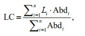
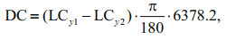
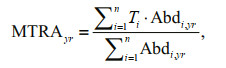
where Abd is the predicted relative abundance, Ti in the equation is the median temperature preference of species i. Details of the three formulas above are referred to Cheung et al.(2013a, b, 2015).
3 RESULT 3.1 Temperature sensitivityIn general, the median preferred temperature of the 17 studied fish species varied widely, ranging from 5 ℃ to 27 ℃, and in curvilinear fashion with the range of the thermal preference, which is calculated from the difference between the temperature corresponding to 95% and 5% percentiles of the cumulative relative abundance for each fish (Fig. 1) (P=0.000 038, R2=0.449 7). This suggests that 17 studied fish tend to be sensitive to temperature changes.

|
| Fig.1 Temperature preference profiles of 17 demersal fishes (source: Fishbase) a. the black circles refer to the median preferred temperature and the lines depict the temperature range corresponding to 95% and 5% percentiles of the cumulative relative abundance of each fish; b. the median thermal preference plotted against the interquartile range of thermal preference. A quadratic curve is fitted to the data points. |
Generally, both sea surface temperature (SST) and sea bottom temperature (SBT) show upward trends during 1970–2060, and the increase of SST is more remarkable. From 1970 to 2060, SST is predicted to rise at an average speed of 0.094 ℃/decade, 0.159 ℃ /decade, and 0.106 ℃/decade in GFDL, IPSL and MPI, respectively, under the RCP 2.6 scenario, while under the RCP 8.5 scenario, SST is predicted to rise at an average speed of 0.194 ℃/decade, 0.297 ℃/ decade and 0.197 ℃/decade, respectively. The ensemble average of SST in three ESMs is predicted to increase by 0.120 and 0.229 ℃/decade under RCP 2.6 and RCP 8.5 scenarios, respectively (Fig. 2). As for SBT between 1970 and 2060, under the RCP 2.6 scenario, it is predicted to rise at an average speed of 0.033, 0.040, and 0.054 ℃/decade in GFDL, IPSL, and MPI respectively, and it is predicted to rise at an average speed of 0.063, 0.042, and 0.058 ℃/decade, respectively, under the RCP 8.5 scenario. Their ensemble average in three ESMs is projected to increase by 0.042 and 0.054 ℃/decade under RCP 2.6 and RCP 8.5 scenarios, during the same period (Fig. 3). Meanwhile, from the spatial perspective, the increasing rate of SST in the northern and coastal regions is more significant than that in the southern and central regions of the Yellow Sea (Fig. 4). For SBT, only the northern area of the Yellow Sea shows a dramatic increase (Fig. 5).

|
| Fig.2 Projected SST between 1970 and 2060 by GFDL, IPSL, MPI under two emission scenarios and its observation |

|
| Fig.3 Projected SBT between 1970 and 2060 by GFDL, IPSL, MPI under two emission scenarios and its observation |

|
| Fig.4 Projected SST changes in 2060 relative to that in 1970 under two emission scenarios (based on GFDL, IPSL, MPI, and their multi-model ensemble) |

|
| Fig.5 Projected SBT changes in 2060 relative to that in 1970 under two emission scenarios (based on GFDL, IPSL, MPI, and their multi-model ensemble) |
As ocean warming induced by increasingatmospheric CO2 concentration, the latitudinal centroids of the 17 demersal species are expected to shift southward in the future. Under the RCP 2.6 scenario, the latitudinal centroids of studied species are projected to shift at an average rate of -8.81±13.19 (standard error, SE), 16.19±12.48, and -12.48±11.04 km/decade with forcing from the Earth system models GFDL, IPSL, and MPI, respectively, between 1970 and 2060 (Fig. 6). At the same time, the corresponding latitudinal centroids were projected to shift at an average rate of -7.59±8.73, 16.01±13.22, and -16.72±14.89 km/decade under the RCP 8.5 scenario (Fig. 6). In comparison, during the same period, the average latitudinal centroids in three ESMs are projected to shift at a rate of -1.17±4.55 and -2.76±3.82 km/decade under the RCP 2.6 and RCP 8.5 scenarios, respectively. (Fig. 6). Though the results modeled by IPSL under both RCP 2.6 and RCP 8.5 scenarios show northward shift, the ensemble means showed an overall trend that the projected latitudinal centroids shift to lower latitudes.

|
| Fig.6 Predicted latitudinal centroids of the 17 demersal fish species in the Yellow Sea under the RCP 2.6 and RCP 8.5 scenarios from 1970 to 2060 that were driven by outputs from GFDL, IPSL, MPI, and ensemble of projections The solid line represents lower and upper limits, the box represents 75% and 25% percentiles while the thick black line represents the median (Positive values represent poleward range shifts). |
The species assemblages in the Yellow Sea may be influenced by anti-poleward distribution shifts (Figs. 7 & 8). In general, the local invasion in the southern area, especially the central part of the southern Yellow Sea, is projected to be more dramatic than that in the northern area under two emission scenarios. At the same time, the local extinction follows the opposite pattern of the local invasion in the Yellow Sea. The local extinction is predicted to be more dramatic in the northern area than in the southern area, and more dramatic in the coastal area than in the central region, under two emission scenarios.

|
| Fig.7 Projected changes in species assemblages represented by the rate of species invasion in 2060 relative to that in 1970 in each 30′×30′ grid under two emission scenarios (based on GFDL, IPSL, MPI, and their multi-model ensemble) |

|
| Fig.8 Projected changes in species assemblages represented by the rate of local extinction in 2060 relative to that in 1970 in each 30′×30′ grid under two emission scenarios (based on GFDL, IPSL, MPI, and their multi-model ensemble) |
Comparison in relative abundance of 17 demersal fishes between 2060 and 1970 under the RCP 2.6 and RCP 8.5 scenarios (Fig. 9) reveals that the relative abundance in the southern region is much higher than that in the northern region in all cases. It is noteworthy that, in the southern Yellow Sea, the relative abundance is much higher in the central part than in its surrounding region.

|
| Fig.9 The projected relative abundance (RA) in 2060 relative to that in 1970 under two emission scenarios (based on GFDL, IPSL, MPI, and their multi-model ensemble) |
According to the projected changes in relative abundance of the 17 demersal fish species, we calculated the mean temperature of relative abundance (MTRA). Generally, the MTRA is expected to grow with the ocean warming from 1970 to 2060 (Fig. 10). The MTRA is predicted to rise by 0.077, 0.065, 0.095 ℃/decade under the RCP 2.6 scenario of GFDL, IPSL, MPI between 1970 and 2060, respectively. At the same time, the MTRA under the RCP 8.5 scenario is predicted to rise by 0.071, 0.062, 0.091 ℃/decade, respectively during the same period.

|
| Fig.10 Calculated MTRA between 1970 and 2060 under the RCP 2.6 and RCP 8.5 scenarios of GLDF, IPSL, and MPI (Green dotted lines represent linear regression fits) |
The species richness is shown in Fig. 11, the numbers of species with positive projected relative abundance in each 30ʹ×30ʹ grid are shown by the color plotted on it. It can be seen from the picture that most of the studied species are predicted to occur in the sea south of 34° latitude. Particularly, under the RCP 8.5 scenario, it is clear that the species. Richness in the central part of southern Yellow Sea is higher than that in its surrounding region.

|
| Fig.11 Predicted species richness of 17 demersal fish species under RCP 2.6 and RCP 8.5 scenarios of GFDL, IPSL, MPI, and their ensemble average in 2060 |
Our results in this study show that 17 demersal fish species in the Yellow Sea would in average shift southward with ocean warming. However, previous studies have reported that most fish species would shift towards the polar or higher latitude with ocean warming (Walther et al., 2002; Perry et al., 2005; Dulvy et al., 2008; Cheung et al., 2015), which are contrary to our findings. The central and southern Yellow Sea displayed coherent patterns in projected SST, relative abundance, and species richness (Figs. 4, 9, & 11), with smaller changes in temperature leading to greater abundance and richness. The specific distributional response might be decided by specific geographical characters and the interactions of currents and water mass in the Yellow Sea.
The Yellow Sea is a marginal sea with an average depth of around 44 m, and its maximum depth is 60–80 m (Wei et al., 2010). Bathymetric contours of the sea illustrate a gradually sloping coast with a relatively deeper trough along the center that has decreasing depths from south to north. This explains why the rising rate of SBT in the central and southern Yellow Sea is significantly lower than that of SST in the same region.
The Asian monsoon system dominates the climate of Yellow Sea. In winter, cold air and strong winds lead to a well-mixed water column, and the surface layer forced by the predominant wind stress flows southward (Naimie et al., 2001). Due to the strong northwesterly wind, the Yellow Sea Coastal Current flows southeastward along the Yangtze Bank (Yuan et al., 2008) and the Korean Coastal Current flows southward along the Korean coast until it meets a thermohaline front (Hsueh, 1988). This thermohaline front forms in the central and southern Yellow Sea (Lie et al., 2013), which have great impacts on the distribution of plankton, provide suitable environmental condition for fish (Liu et al., 2015; Mei et al., 2016). Due to the unique and complex bottom topography combined with the summer meteorological forcing, cold waters from the previous winter are locally trapped in a topographic depression after the onset of seasonal stratification, resulting in a large cold water mass to persist in the deep basin, which is called the Yellow Sea Bottom Cold Water or the Yellow Sea Cold Water Mass (Hur et al., 2000; Wei et al., 2010; Yuan et al., 2013). The Yellow Sea Cold Water Mass is one of the most prominent summer oceanographic phenomena in the Yellow Sea, which have a great impact on phytoplankton biomass and zooplankton distributions (Chen et al., 2004). Meanwhile, it slows down the rate of ocean warming in the southern Yellow Sea (Jiang et al., 2007; Li et al., 2017).
In summary, topography, currents, and water masses together result in better conditions for the survival and development of demersal fish species in the central and southern Yellow Sea, leading to its southward distributional response. Furthermore, as it is shown in Figs. 7 & 8, the different ocean warming rate in the Yellow Sea would also trigger local extinction in northern area and species invasion in southern area, which may change the community structure in the Yellow Sea, so this finding would provide important implications for fishery resource management and conservation.
4.2 Temperature variationIn contrast to the significant increase of SST, the projected increasing rate of SBT in the central and southern Yellow Sea is weaker (Fig. 5). In this case, the southward migration of the studied species can be explained as their vulnerability to temperature changes. It is reported that demersal fish tended to be more vulnerable to climate change than pelagic fishes (Chen et al., 2019). Demersal fishes usually have large body size, which is associated with complex population structure, low fecundity, and slow intrinsic population growth rate (Denney et al., 2002).
Demersal fishes with these characteristics, which are influenced by multiple threats, are more susceptible to environmental changes such as ocean deoxygenation and seawater warming leading to a low adaptability to climate change (Chen et al., 2019). Moreover, the mean temperature of relative abundance (MTRA) of studied species (Fig. 10) increases consistently from 1970 to 2060 in both modelling outputs under the RCP 2.6 and RCP 8.5 scenarios. MTRA was calculated with reference to mean temperature of the catch (MTC) in the study of Cheung et al. (2013b) and fishery catch is replaced by projecting relative abundance. The growth of MTRA indicates that living temperature of the 17 demersal fishes is still increasing with their southward distributional response. It has been reported that the net SST of the Yellow Sea increased by 0.678 ℃ from 1982 to 2006, higher than the global mean (Belkin, 2009). Once the increase in the prevailing temperature, in the Yellow sea cold water mass, exceeds the preferred range of temperature for demersal fish, it is expected to lead substantial change in population structure. Therefore, besides the direct measures such as marine ranching construction and fishing ground conservation, measures curbing ocean warming are also urgently needed to preserve fishery resources.
4.3 Model limitationIn this study, distributions of demersal fish species were modeled based on the correspondence between species distribution and environmental variables. In DBEM, projecting spatial distribution is subject to both population dynamic characteristics and the relation between environmental conditions and species occurrence. By associating occurrence data with current environmental variables, environmental envelopes were calculated to find the absolute and "preferred" preference ranges (Kaschner et al., 2011; Jones et al., 2012). Given the ecological and biological characteristics of each species, the relative environmental suitability of the habitat to the affinity of each species was transformed into values in a cell ranging from 0 and 1 (Cheung et al., 2013b). This method has some inherent defects. For example, it cannot take evolutionary or ecological parameters that could refine such distribution into consideration (e.g. adaptation; interspecific interactions; changes in other trophic levels).
The availability of surveyed or observed data makes tracking long-term changes in distribution and abundance of fish challenging. The DBEM and ESMs applied in this paper allow to predict changes in distribution and relative abundance of demersal fish species in the Yellow Sea by accounting species preferred environmental habitat, overcoming the limited data availability. In addition, surveyed or observed data in the Yellow Sea is not enough to exam the projecting results. There are some uncertainties in DBEM, including (i) structural (model) uncertainty, (ii) parametric uncertainty, (iii) initialization and internal variability uncertainty, and (iv) scenario uncertainty; for example, the occurrence of species invasions in the northern region with GFDL under RCP 8.5 in Fig. 7 reflects the limitation and uncertainty of this method, but several studies in other areas have proved the reliability of this method (Cheung et al., 2015, 2016a; Frölicher et al., 2016; Payne et al., 2016), so the general trends revealed from the analysis should be robust. In addition, estimates of climate changes were obtained from the outputs of global ESMs with a coarse resolution, whereas the present study was conducted on a regional scale. So it is necessary to develop higher-resolution regional models with more regional biogeochemical characters to provide more detailed predictions about ocean variables.
5 CONCLUSIONThe southward distributional response of 17 demersal fish species under climate change is revealed by DBEM and ESMs in this paper. The main reasons for this phenomenon are the semi-enclosed topography of the Yellow Sea and the interaction between ocean currents and water masses, especially the Yellow Sea Cold Water Mass. This finding provides a better understanding of potential pattern of fish stock and distribution shifts under possible climate change scenarios, and suggests the urgency of curbing ocean warming.
6 DATA AVAILABILITY STATEMENTThe data that support the findings of this study are openly available in Science at https://doi.org/10.1126/science.aag2331, reference (Cheung et al., 2016b). The data that support the findings of this study are openly available in FishBase at https://www.fishbase.org, the Oceanic Biogeographic Information System at http://iobis.org, SeaLifeBase at https://www.sealifebase.org, and Sea Around Us Project at https://www.seaaroundus.org.
Baudron A R, Needle C L, Rijnsdorp A D, Marshall C T. 2013. Warming temperatures and smaller body sizes: synchronous changes in growth of North Sea fishes. Global Change Biology, 20(4): 1023-1031.
DOI:10.1111/gcb.12514 |
Belkin I M. 2009. Rapid warming of large marine ecosystems. Progress in Oceanography, 81(1-4): 207-213.
DOI:10.1016/j.pocean.2009.04.011 |
Calbet A, Sazhin A F, Nejstgaard J C, Berger S A, Tait Z S, Olmos L, Sousoni D, Isari S, Martínez R A, Bouquet J M, Thompson E M, Båmstedt U, Jakobsen H H. 2014. Future climate scenarios for a coastal productive planktonic food web resulting in microplankton phenology changes and decreased trophic transfer efficiency. PLoS One, 9(4): e94388.
DOI:10.1371/journal.pone.0094388 |
Chen Y L, Hu D X, Wang F. 2004. Long-term variabilities of thermodynamic structure of the East China Sea Cold Eddy in summer. Chinese Journal of Oceanology and Limnology, 22(3): 224-230.
DOI:10.1007/BF02842552 |
Chen Y L, Shan X J, Wang N, Jin X S, Guan L S, Gorfine H, Yang T, Dai F Q. 2019. Assessment of fish vulnerability to climate change in the Yellow Sea and Bohai Sea. Marine and Freshwater Research, 71(7): 729-736.
DOI:10.1071/MF19101 |
Cheung W W L, Brodeur R D, Okey T A, Pauly D. 2015. Projecting future changes in distributions of pelagic fish species of Northeast Pacific shelf seas. Progress in Oceanography, 130: 19-31.
DOI:10.1016/j.pocean.2014.09.003 |
Cheung W W L, Dunne J P, Sarmiento J L, Pauly D. 2011. Integrating ecophysiology and plankton dynamics into projected maximum fisheries catch potential under climate change in the Northeast Atlantic. ICES Journal of Marine Science, 68(6): 1008-1018.
DOI:10.1093/icesjms/fsr012 |
Cheung W W L, Jones M C, Reygondeau G, Stock C A, Lam V W Y, Frölicher T L. 2016a. Structural uncertainty in projecting global fisheries catches under climate change. Ecological Modelling, 325: 57-66.
DOI:10.1016/j.ecolmodel.2015.12.018 |
Cheung W W L, Lam V W Y, Pauly D. 2008. Dynamic bioclimate envelope model to predict climate-induced changes in distribution of marine fishes and invertebrates. In: Cheung W W L, Lam V W Y, Pauly D eds. Modelling Present and Climate-shifted Distribution of Marine Fishes and Invertebrates. University of British Columbia, Canada. p. 5-50.
|
Cheung W W L, Lam V W Y, Sarmiento J L, Kearney K, Watson R, Pauly D. 2009. Projecting global marine biodiversity impacts under climate change scenarios. Fish and Fisheries, 10(3): 235-251.
DOI:10.1111/j.1467-2979.2008.00315.x |
Cheung W W L, Reygondeau G, Frölicher T L. 2016b. Large benefits to marine fisheries of meeting the 1.5¦ global warming target. Science, 354(6319): 1591-1594.
DOI:10.1126/science.aag2331 |
Cheung W W L, Sarmiento J L, Dunne J, Frölicher T L, Lam V W Y, Deng Palomares M L, Watson R, Pauly D. 2013a. Shrinking of fishes exacerbates impacts of global ocean changes on marine ecosystems. Nature Climate Change, 3(3): 254-258.
DOI:10.1038/nclimate1691 |
Cheung W W L, Watson R, Pauly D. 2013b. Signature of ocean warming in global fisheries catch. Nature, 497(7449): 365-368.
DOI:10.1038/nature12156 |
Close C H, Cheung W W L, Hodgson S, Lam V, Watson R, Pauly D. 2006. Distribution ranges of commercial fishes and invertebrates. In: Palomares M L D, Stergiou K I, Pauly D eds. Fishes in Databases and Ecosystems. Fisheries Centre Research Report. University of British Columbia, Vancouver. p. 27-37.
|
Dai F Z, Zhu L, Chen Y L. 2020. Variations of fishery resource structure in the Yellow Sea and East China Sea. Progress in Fishery Sciences, 41(1): 1-10.
DOI:10.19663/j.issn2095-9869.20181120001. |
Denney N H, Jennings S, Reynolds J D. 2002. Life-history correlates of maximum population growth rates in marine fishes. Proceedings of the Royal Society B: Biological Sciences, 269(1506): 2229-2237.
DOI:10.1098/rspb.2002.2138 |
Dulvy N K, Rogers S I, Jennings S, Stelzenmüller V, Dye S R, Skjoldal H R. 2008. Climate change and deepening of the North Sea fish assemblage: a biotic indicator of warming seas. Journal of Applied Ecology, 45(4): 1029-1039.
DOI:10.1111/j.1365-2664.2008.01488.x |
Edwards M, Richardson A J. 2004. Impact of climate change on marine pelagic phenology and trophic mismatch. Nature, 430(7002): 881-884.
DOI:10.1038/nature02808 |
Frölicher T L, Rodgers K B, Stock C A, Cheung W W L. 2016. Sources of uncertainties in 21st century projections of potential ocean ecosystem stressors. Global Biogeochemical Cycles, 30(8): 1224-1243.
DOI:10.1002/2015GB005338 |
Golden C D, Allison E H, Cheung W W L, Dey M M, Halpern B S, McCauley D J, Smith M, Vaitla B, Zeller D, Myers S S. 2016. Nutrition: fall in fish catch threatens human health. Nature, 534(7607): 317-320.
DOI:10.1038/534317a |
Harley C D G. 2011. Climate change, keystone predation, and biodiversity loss. Science, 334(6059): 1124-1127.
DOI:10.1126/science.1210199 |
Hsueh Y. 1988. Recent current observations in the eastern Yellow Sea. Journal of Geophysical Research: Oceans, 93(C6): 6875-6884.
DOI:10.1029/JC093iC06p06875 |
Huang J S, Sun Y, Jia H B, Yang Q, Tang Q S. 2014. Spatial distribution and reconstruction potential of Japanese anchovy (Engraulis japonicus) based on scale deposition records in recent anaerobic sediment of the Yellow Sea and East China Sea. Acta Oceanologica Sinica, 33(12): 138-144.
DOI:10.1007/s13131-014-0573-8 |
Hur H B, Jacobs G A, Teague W J. 2000. Monthly variations of water masses in the Yellow and East China Seas. Journal of Oceanography, 56(3): 359.
DOI:10.1023/A:1011163919440 |
Jiang B J, Bao X W, Wu D X, Xu J P. 2007. Interannual variation of temperature and salinity of northern Huanghai Sea Cold Water Mass and its probable cause. Acta Oceanologica Sinica, 29(4): 1-10.
DOI:10.3321/j.issn:0253-4193.2007.04.001. |
Jin X S, Tang Q S. 1996. Changes in fish species diversity and dominant species composition in the Yellow Sea. Fisheries Research, 26(3-4): 337-352.
DOI:10.1016/0165-7836(95)00422-X |
Jones M C, Dye S R, Pinnegar J K, Warren R, Cheung W W L. 2012. Modelling commercial fish distributions: prediction and assessment using different approaches. Ecological Modelling, 225: 133-145.
DOI:10.1016/j.ecolmodel.2011.11.003 |
Kaschner K, Tittensor D P, Ready J, Gerrodette T, Worm B. 2011. Current and future patterns of global marine mammal biodiversity. PLoS One, 6(5): e19653.
DOI:10.1371/journal.pone.0019653 |
Kwiatkowski L, Bopp L, Aumont O, Ciais P, Cox P M, Laufkötter C, Li Y, Séférian R. 2017. Emergent constraints on projections of declining primary production in the tropical oceans. Nature Climate Change, 7(5): 355-358.
DOI:10.1038/nclimate3265 |
Laufkötter C, Vogt M, Gruber N, Aita-Noguchi M, Aumont O, Bopp L, Buitenhuis E, Doney S C, Dunne J, Hashioka T, Hauck J, Hirata T, John J, Le Quéré C, Lima I D, Nakano H, Seferian R, Totterdell I, Vichi M, Völker C. 2015. Drivers and uncertainties of future global marine primary production in marine ecosystem models. Biogeosciences, 12(23): 6955-6984.
DOI:10.5194/bg-12-6955-2015 |
Lefort S, Aumont O, Bopp L, Arsouze T, Gehlen M, Maury O. 2015. Spatial and body-size dependent response of marine pelagic communities to projected global climate change. Global Change Biology, 21(1): 154-164.
DOI:10.1111/gcb.12679 |
Li A, Yu F, Si G C, Wei C J. 2017. Long-term temperature variation of the Southern Yellow Sea Cold Water Mass from 1976 to 2006. Chinese Journal of Oceanology and Limnology, 35(5): 1032-1044.
DOI:10.1007/s00343-017-6037-1 |
Li Z L, Shan X J, Jin X S, Dai F Q. 2011. Long-term variations in body length and age at maturity of the small yellow croaker(Larimichthys polyactis Bleeker, 1877) in the Bohai Sea and the Yellow Sea, China. Fisheries Research, 110(1): 67-74.
DOI:10.1016/j.fishres.2011.03.013 |
Lie H J, Cho C H, Lee S. 2013. Frontal circulation and westward transversal current at the Yellow Sea entrance in winter. Journal of Geophysical Research: Oceans, 118(8): 3851-3870.
DOI:10.1002/jgrc.20280 |
Liu X, Huang B Q, Huang Q, Wang L, Ni X B, Tang Q S, Sun S, Wei H, Liu S M, Li C L, Sun J. 2015. Seasonal phytoplankton response to physical processes in the southern Yellow Sea. Journal of Sea Research, 95: 45-55.
DOI:10.1016/j.seares.2014.10.017 |
Mei X, Li R H, Zhang X H, Liu Q S, Liu J X, Wang Z B, Lan X H, Liu J, Sun R T. 2016. Evolution of the Yellow Sea Warm Current and the Yellow Sea Cold Water Mass since the Middle Pleistocene. Palaeogeography, Palaeoclimatology, Palaeoecology, 442: 48-60.
DOI:10.1016/j.palaeo.2015.11.018 |
Miloslavich P, Bax N J, Simmons S E, Klein E, Appeltans W, Aburto-Oropeza O, Andersen Garcia M, Batten S D, Benedetti-Cecchi L, Checkley D M, Chiba S, Duffy J E, Dunn D C, Fischer A, Gunn J, Kudela R, Marsac F, Muller-Karger F E, Obura D, Shin Y J. 2018. Essential ocean variables for global sustained observations of biodiversity and ecosystem changes. Global Change Biology, 24(6): 2416-2433.
DOI:10.1111/gcb.14108 |
Naimie C E, Blain C A, Lynch D R. 2001. Seasonal mean circulation in the Yellow Sea-a model-generated climatology. Continental Shelf Research, 21(6-7): 667-695.
DOI:10.1016/S0278-4343(00)00102-3 |
Payne M R, Barange M, Cheung W W L, Mackenzie B R, Batchelder H P, Cormon X, Eddy T D, Fernandes J A, Hollowed A B, Jones M C, Link J S, Neubauer P, Ortiz I, Queirós A M, Paula J R. 2016. Uncertainties in projecting climate-change impacts in marine ecosystems. ICES Journal of Marine Science, 73(5): 1272-1282.
DOI:10.1093/icesjms/fsv231 |
Perry A L, Low P J, Ellis J R, Reynolds J D. 2005. Climate change and distribution shifts in marine fishes. Science, 308(5730): 1912-1915.
DOI:10.1126/science.1111322 |
Pinsky M L, Worm B, Fogarty M J, Sarmiento J L, Levin S A. 2013. Marine taxa track local climate velocities. Science, 341(6151): 1239-1242.
DOI:10.1126/science.1239352 |
Reygondeau G, Maury O, Beaugrand G, Fromentin J M, Fonteneau A, Cury P. 2012. Biogeography of tuna and billfish. Journal of Biogeography, 39(1): 114-129.
DOI:10.1111/j.1365-2699.2011.02582.x |
Sheridan J A, Bickford D. 2011. Shrinking body size as an ecological response to climate change. Nature Climate Change, 1(8): 401-406.
DOI:10.1038/nclimate1259 |
Simpson S D, Jennings S, Johnson M P, Blanchard J L, Schön P J, Sims D W, Genner M J. 2011. Continental shelf-wide response of a fish assemblage to rapid warming of the Sea. Current Biology, 21(18): 1565-1570.
DOI:10.1016/j.cub.2011.08.016 |
Walther G R, Post E, Convey P, Menzel A, Parmesan C, Beebee T J C, Fromentin J M, Hoegh-Guldberg O, Bairlein F. 2002. Ecological responses to recent climate change. Nature, 416(6879): 389-395.
DOI:10.1038/416389a |
Wei H, Shi J, Lu Y Y, Peng Y. 2010. Interannual and long-term hydrographic changes in the Yellow Sea during 1977-1998. Deep Sea Research Part II: Topical Studies in Oceanography, 57(11-12): 1025-1034.
DOI:10.1016/j.dsr2.2010.02.004 |
Xu B D, Jin X S, Liang Z L. 2003. Changes of demersal fish community structure in the Yellow Sea during the autumn. Journal of Fishery Sciences of China, 10(2): 148-154.
DOI:10.3321/j.issn:1005-8737.2003.02.013 |
Xu B D, Jin X S. 2005. Variations in fish community structure during winter in the southern Yellow Sea over the period 1985-2002. Fisheries Research, 71(1): 79-91.
DOI:10.1016/j.fishres.2004.07.011 |
Yuan D L, Li Y, Qiao F L, Zhao W. 2013. Temperature inversion in the Huanghai Sea bottom cold water in summer. Acta Oceanologica Sinica, 32(3): 42-47.
DOI:10.1007/s13131-013-0287-3 |
Yuan D L, Zhu J R, Li C Y, Hu D X. 2008. Cross-shelf circulation in the Yellow and East China Seas indicated by MODIS satellite observations. Journal of Marine Systems, 70(1-2): 134-149.
DOI:10.1016/j.jmarsys.2007.04.002 |
Zhang B, Tang Q S. 2004. Study on trophic level of important resources species at high troph levels in the Bohai Sea, Yellow Sea and East China Sea. Advances in Marine Science, 22(4): 393-404.
DOI:10.3969/j.issn.1671-6647.2004.04.001. |
Zhao X, Hamre J, Li F, Jin X, Tang Q. 2003. Recruitment, sustainable yield and possible ecological consequences of the sharp decline of the anchovy (Engraulis japonicus)stock in the Yellow Sea in the 1990s. Fisheries Oceanography, 12(4-5): 495-501.
DOI:10.1046/j.1365-2419.2003.00262.x |