 2022, Vol. 40
Institute of Oceanology, Chinese Academy of Sciences
Article Information
- QU Baoxiao, SONG Jinming, LI Xuegang, YUAN Huamao, ZHANG Kun, XU Suqing
- Global air-sea CO2 exchange flux since 1980s: results from CMIP6 Earth System Models
- Journal of Oceanology and Limnology, 40(4): 1417-1436
- http://dx.doi.org/10.1007/s00343-021-1096-8
Article History
- Received Apr. 8, 2021
- accepted in principle May 8, 2021
- accepted for publication Oct. 4, 2021


2 Marine Ecology and Environmental Sciences Laboratory, Pilot National Laboratory for Marine Science and Technology (Qingdao), Qingdao 266237, China;
3 University of Chinese Academy of Sciences, Beijing 100049, China;
4 Center for Ocean Mega-Science, Chinese Academy of Sciences, Qingdao 266071, China;
5 Key Laboratory of Ocean Circulation and Waves, Institute of Oceanology, Chinese Academy of Sciences, Qingdao 266071, China;
6 Key Laboratory of Global Change and Marine-Atmospheric Chemistry, Third Institute of Oceanography, Ministry of Natural Resources, Xiamen 361005, China
According to the Fifth Intergovernmental Panel on Climate Change (IPCC) Assessment Report, the concentration of carbon dioxide (CO2) in the atmosphere has increased by about 40% from 278×10-6 in 1750 to 390×10-6 in 2011 (Ciais et al., 2013). The Fifth Report also stated, during the same period, about 555±85 Pg C (1 Pg=1015 g) anthropogenic CO2 had ever been released into the atmosphere. And about 28% of them had been absorbed by the ocean (155±85 Pg C). The exchange flux of CO2 between the atmosphere and ocean, therefore, could significantly moderate the negative impact of greenhouse effect caused by increasing atmospheric CO2 concentration, and then profoundly affect the future trajectory of global climate change. Methodologically, the air-sea CO2 exchange flux could be obtained by both observation-based estimations (Takahashi et al., 2002; Key et al., 2004; Sweeney et al., 2007; Rödenbeck et al., 2015) and model simulation outputs (Le Quéré et al., 2000; Fletcher et al., 2006; Li and Xu, 2012, 2013; Luo et al., 2015; Wang et al., 2015). But in a way, model simulation can compensate for the inevitable temporal-spatial limitation of observation-based methods. Consequently, numerical models are widely used to study the feature and variability of global air-sea CO2 exchange process. The Earth System Models (ESMs) are the latest generation of the state-of-the-art climate models, which couple the carbon cycle processes among the atmosphere, land, and ocean, and simulate the real earth systems to the maximum extent. Therefore, the ESMs could serve as a helpful and powerful tool to analyze and diagnose the global carbon cycles.
The Coupled Model Intercomparison Project (CMIP) standardizes the ESMs' outputs in a specified format and makes their results publicly available, in order to better understand the past, present, and future climate change arising from both natural and anthropogenic forcing. Anav et al. (2013) evaluated the results of ESMs in the fifth phase of CMIP (CMIP5), and found most of them shown an acceptable skill for the global air-sea CO2 flux simulation. Their ensemble average flux increased almost by three times from a sink of 0.56±0.13 Pg C/a during the period 1900–1930 to 1.6±0.2 Pg C/a during the period 1960–2005. Furthermore, the ESMs highlighted the significance of the Southern Ocean for the global anthropogenic CO2 budget (Frölicher et al., 2015), which had absorbed 42±5 Pg C of anthropogenic CO2 over the 1860 to 2005 period. However, the models also have their own deficiency. More than half of the ESMs included in CMIP5 could hardly reproduce the spatial pattern of the tropical Pacific CO2 flux during El Niño events, despite their reasonable performances in the simulation of the mean states (Dong et al., 2016, 2017; Jin et al., 2019).
The latest CMIP has moved ahead into the sixth phase (CMIP6, Eyring et al., 2016) and how do the up-to-date datasets simulated by the new versions of ESMs characterize the temporal and spatial variabilities of the global air-sea CO2 flux? Could they describe the global oceanic CO2 source/sink pattern more reasonably? In order to answer these questions, description and evaluation of the Coupled Model Intercomparison Project Phase 6 (CMIP6) ESMs and their related datasets are important and imperative. This paper presents the background information of the new version of CMIP ESMs, provides their results of air-sea CO2 exchange flux (FCO2), and estimates the long-term average, interannual variability and historical tendency of them. The remainder of this paper is organized as following. Section 2 introduces the models, datasets, and analytical methods. The results are presented in Section 3. Section 4 discusses the main controlling processes and Section 5 makes the conclusion.
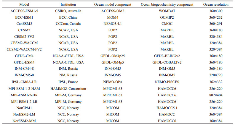
2 MATERIAL AND METHODEighteen CMIP6 Earth System Models were adopted in this article. Their names, sources, components, resolutions were summarized in Table 1. The related FCO2 results were derived from the "historical" experiment of each model, which were forced by the historical atmospheric CO2 concentration over the period 1850 to 2014 (Eyring et al., 2016). These CMIP6 FCO2 results were obtained from the public data portals of the Earth System Grid Federation (https://esgf-node.llnl.gov/projects/cmip6/). We adopt the variable of "fgco2" in every CMIP6 model, which means "surface downward mass flux of carbon dioxide expressed as carbon", to evaluate the air-sea CO2 exchange flux.
Observational datasets employed in this paper included the climatological FCO2 for a reference year 2000 from Lamont-Doherty Earth Observatory of Columbia University with a resolution of 4°×5° (Takahashi et al., 2009). We referred it as "Takahashi2009" and re-gridded it into the 1°×1° grid for the comparisons of long-term FCO2 average and spatial distributions of model biases. The observational monthly FCO2 was derived from Landschützer et al.(2016, 2017) which was developed by a neural network technology with a resolution of 1°×1° and a time span from 1982 to 2014. We referred it as "Landschützer2017" in this study to assess the spatial-temporal variabilities and historical tendencies of FCO2. To evaluate the performance of FCO2 simulations in these CMIP6 ESMs quantitatively, root-mean-square error (RMSE) and the normalized standard deviation were calculated. RMSE illustrates the mean-state deviation of the model simulation from the observation, and the normalized standard deviation reflects the interannual variation of air-sea CO2 exchange flux.
3 RESULT 3.1 Global long-term averageThe simulated global long-term average of air-sea CO2 flux in CMIP6 ESMs are compared with the observational results of Takahashi2009 (Fig. 1 and Supplementary Fig.S1). All the selected models could generally reproduce the dominant patterns of Takahashi2009: the equatorial Pacific is the major oceanic CO2 source for atmosphere, the temperate oceans in both hemispheres are the major oceanic sinks for atmospheric CO2, and the North Atlantic is the most intensive CO2 sink (Supplementary Fig.S1). These consistent results imply the selected CMIP6 ESMs performance fairly good in simulating the climatological state of global air-sea CO2 exchange process. Nevertheless, there are some divergences between the modeled FCO2 and the observed FCO2 in individual models. For instance, most models do not capture or just underestimate the release of CO2 in Bering Sea, except GFDL-CM4 and GFDL-ESM4. Two models, namely INM-CM4-8 and INM-CM5-0, seemed to give extra weight to the Southern Ocean in oceanic CO2 outgassing, and one model, namely BCC-ESM1 overestimated the CO2 sink in the high latitude region of Southern Ocean (south of 60°S).

|
| Fig.1 The air-sea CO2 flux climatology for the observationally based results of Takahashi2009 (a) (units: 10-9 kg C/(m2∙s)); model biases with respect to the result of Takahashi2009 (b–s) (model results minus Takahashi2009 results) Positive value means the ocean releases CO2 into the atmosphere and negative value mean ocean absorbs CO2 from the atmosphere. |
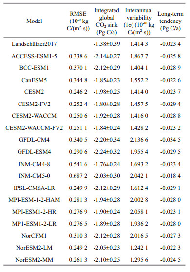
We further calculated the RMSE to assess the longterm state of air-sea CO2 flux in CMIP6 ESMs simulations respect to the observation result of Landschützer2017 during the period of 1982–2014 (Table 2). In general, most of the CMIP6 ESMs but INM-CM4-8 and INM-CM5-0 have quite low RMSE respect to the Landschützer2017. This implies a fact that most of the selected CIMP6 ESMs have good performance in simulating the long-term state of FCO2. It should be pointed out that four models from the National Center for Atmospheric Research of USA, namely CESM2, CESM2-FV2, CESM-WACCM, CESM-WACCM-FV2, and two models from the NorESM Climate Modeling Consortium, namely NorESM2-LM, NorESM2-MM, performed particularly well because their RMSE results were generally confined to the range of 0.2400 to 0.2600.
|
Basing on the CMIP6 simulated FCO2 datasets, we examined the time series of integrated global FCO2 during from 1850 to 2014 (Fig. 2) and calculated the long-term averages of integrated FCO2 basing on the results from 1982 to 2014 (Table 2) for each model. We found that, before 1950s, the global ocean (the results of INM-CM4-8 and INM-CM5-0 were excluded because of their poor performances) generally behaves as a moderate CO2 sink with the flux about -0.5 Pg C/a (Fig. 2). However, after 1950s, the intensity of the oceanic CO2 sink has obviously increased (Fig. 2). If we just focus on the time after 1980s, we could find that the models generally show apparent consistency for the global air-sea CO2 flux (Fig. 2). The CMIP6 ESMs simulated long-term average intergrated global CO2 sink in recent three decades ranges from 1.80 to 2.24 Pg C/a (Table 2). This value is somewhat higher than the previous study, e.g., 1.48 Pg C/a from Valsala and Maksyutov (2010), 1.42±0.53 Pg C/a from Landschützer et al. (2014), 1.8±0.7 from Doney et al. (2009) and 2.0±1 Pg C/a from Takahashi et al. (2009), but very close to the result of Zeng et al. (2014) (1.9 to 2.3 Pg C/a). In consideration of that there were some inevitable divergences in data arrangement and concerned period between the CMIP6 ESMs and previous studies, the CMIP6 ESMs simulated integrated global air-sea CO2 flux could be supposed to consistent with previous results in the term of longtime average. Illustrated by Fig. 2, the observation-based result of Landschützer2017 experienced significant fluctuation during the period of 1980s-2010s. Specifically, before 2000 the global oceanic CO2 sink showed a anomalous decreasing trend of about 0.025 4 Pg C/a. And after 2000 the CO2 sink increased profoundly as high as 0.081 9 Pg C/a. However, this drastic variation is not reflected by any of the selected eighteen CMIP6 ESMs. The possible reasons about this discrepancy would be discussed in the following sections.

|
| Fig.2 Time-series of global integrated air-sea CO2 flux (Pg C/a) for eighteen CMIP6 ESMs and the result of Landschützer2017 |
We concern the air-sea CO2 exchange flux not only on the global scale but on the biogeochemical province scales. For the convenience of comparison, the global open-ocean biomes defined by Fay and McKinley (2014) are adopted in this study. To simplify, some of the smaller biomes within each basin are put together. In this way, we roughly divide the global ocean into ten open-sea biomes: (a) the Indian Ocean, (b) the North Atlantic, (c) the North Pacific, (d) the Southern Ocean, (e) the tropical Atlantic, (f) the temperate Atlantic (North Hemisphere), (g) the temperate Atlantic (South Hemisphere), (h) the temperate Pacific (North Hemisphere), (i) the temperate Pacific (South Hemisphere), and (j) the tropical Pacific (Fig. 3). These ten regions generally cover the global ocean with the exception of the Arctic Ocean and few marginal seas just like the practices of Landschützer et al.(2016, 2017). To assess the performance of every CMIP6 ESMs in simulating the FCO2 for different biomes, we plotted the Taylor diagram of simulated FCO2 comparing with the result of Landschützer2017 for the ten open-ocean biomes during from 1982 to 2014 (Fig. 4). The Taylor diagram could illustrate how well the models output match with the observation result by displaying the spatial correlation coefficient (COR), the standard deviation (STD), and the RMSE in a single two-dimensional diagram (Taylor, 2001). In the following paragraphs, we will present the diversities of CMIP6 ESMs simulated FCO2 in different open-sea biomes.

|
| Fig.3 The ten open-sea biomes of the global ocean |

|
| Fig.4 The Taylor diagrams for CMIP6 ESMs simulated long-term average FCO2 (1982–2014) comparing with the result of Landschützer2017 in the ten open-ocean biomes The black coordinate axis indicates normalized standard deviation, the blue coordinate axis indicates spatial correlation coefficient, and the green coordinate axis indicates the normalized centered RMSE. In each diagram, the black dot stands for the result of Landschützer2017 as the reference, and the red dots stand for the statistics results of each CMIP6 ESM. The data was derived from 18 CMIP6 ESMs. The responding CMIP6 ESMs are (1) ACCESS-ESM1-5; (2) BCC-ESM1; (3) CanESM5; (4) CESM2; (5) CESM2-FV2; (6) CESM2-WACCM; (7) CESM2-WACCM-FV2; (8) GFDL-CM4; (9) GFDL-ESM4; (10) INM-CM4-8; (11) INM-CM5-0; (12) IPSL-CM6A-LR; (13) MPI-ESM-1-2-HAM; (14) MPI-ESM1-2-HR; (15) MPI-ESM1-2-LR; (16) NorCPM1; (17) NorESM2-LM; (18) NorESM2-MM. |
The detailed Taylor diagram is presented in Fig. 4 to quantitatively assess the individual performance of eighteen CMIP6 ESMs in the simulation of long-term (1982–2014) mean state air-sea CO2 exchange flux. Better simulation performance is indicated by a higher spatial correlation coefficient and a low RMSE. The ten open-sea biomes we divided could be broadly classified into two groups. The normal group includes the Indian Ocean, the North Pacific, the Southern Ocean, the temp Atlantic (both hemisphere), and the temp Pacific (both hemisphere). In these seven biomes, the divergence among different CMIP6 ESMs' performance is relatively small (except for very few special situations, such as the INM-CM4-8 and INM-CM5-0), suggesting the consistency of these models in simulating the basin-scale long-term mean state of air-sea CO2 exchange process (Fig. 4a & c–i). The extraordinary group includes the North Atlantic, the tropical Atlantic, and the tropical Pacific. In these three biomes, the divergence among different CMIP6 ESMs' performance is comparatively large. For example, in the North Atlantic, all of the normalized RMSE and STD are larger than 1.0. And the spatial correlation coefficients of ACCESS-ESM1-5, BCC-ESM1, CanESM5, and GFDL-CM4 are lower than 0.4. The above findings jointly indicate the simulation skill of air-sea CO2 exchange process in CMIP6 ESMs is defectively in the North Atlantic. As for the tropical Atlantic and tropical Pacific, the results of RMSE, and STD are distributed dispersedly in the Taylor diagrams (Fig. 4e & i), suggesting the simulation performance of CMIP6 ESMs on FCO2 are quite heterogeneous in these two tropical biomes. GFDL-CM4 and BCC-ESM1 have the highest STD in the tropical Atlantic and tropical Pacific, respectively. Furthermore, more than half of the whole models have spatial correlation coefficient lower than 0.5.
3.3 Interannual variabilityIn this section, the interannual variability of FCO2 during from 1982 to 2014 was assessed by the standard deviation (1σ, STD), which was calculated after detrending and deseasoning, to remove the long-term and seasonal signals. As for observation, the global mean interannual variability is 1.414 3 (Table 2, Landschützer2017, units: 10-10 kg C/(m2·s), the same below). We compare this value with the CMIP6 ESMs' results and find the STD between models and observation show large spread (from 1.242 1 for the NorESM2-LM to 2.136 6 for the GFDL-CM4). There are six models, including BCC-ESM1, CESM2, CESM2-WACCM, CESM2-WACCM-FV2, NorESM2-LM, and NorESM2-MM, possessing lower or comparative interannual variability relative to the observation. And another eight models, including ACCESS-ESM1-5, GFDL-CM4, GFDL-ESM4, INM-CM5-0, MPI-ESM-1-2-HAM, MPI-ESM1-2-HR, MPI-ESM1-2-LR, and NorCPM1 have relatively high interannual variability (STD > 1.800, Table 2).
Basing on the observation data of Landschützer 2017, we find there are two kinds of ocean regions which possess high interannual variability. One is the high latitude regions in both hemispheres, such as the North Pacific, the North Atlantic, and the Southern Ocean (Fig. 5a). Another important region with high interannual variability is the tropical Pacific (Fig. 5a). In order to assess the simulation performance of CMIP6 ESMs in reproducing the interannual variability of global air-sea CO2 flux, we calculated the ratio of STD between model and observation. As for the high latitude oceans in north hemisphere, most models could capture the observed intensive interannual variability because the ratios of standard deviation between CMIP6 ESMs and Landschützer2017 are distributed around 1.0. However, as for the Southern Ocean, the correspondingly ratios are extremely high in the models of INM-CM4-8, INM-CM5-0, MPI-ESM-1-2-HAM, MPI-ESM1-2-HR, MPI-ESM1-2-LR, and NorCPM1 (Figs. 5k–l & n–q), implying these six CMIP6 ESMs are insufficient in reproducing the interannual variability of FCO2 in the Southern Ocean. In the term of tropical ocean, what' more, almost all of the CMIP6 ESMs (except INM-CM4-8 and INM-CM5-0) have presented abnormally high interannual variabilities of FCO2 in Eastern Indian Ocean and tropical Western Pacific (namely the tropical Indo-Pacific Ocean). In addition, ACCESS-ESM1-5, BCC-ESM1, CESM2, CESM2-FV2, CESM2-WACCM, CESM2-WACCM-FV2, GFDL-CM4, GFDL-ESM4 and NorCPM1 also have simulated abnormally high interannual variabilities of FCO2 in the eastern tropical Pacific (Figs. 5b–c, e–j, & q).

|
| Fig.5 The interannual variability of observed FCO2 (10-10 kg C/(m2·s)) during 1982–2014 basing on the standard deviation of monthly data for Landschützer2017 (a); the ratios of standard deviation between the model and observations (b–s) To remove long-term and seasonal signal, the original FCO2 are detrended and deseasoned. |
The historical tendency of CMIP6 ESMs modeled FCO2 since 1980s is evaluated and discussed in this section (Fig. 6 and Table 2). In the term of global integrated air-sea FCO2, the results of CMIP6 ESMs indicate an common decrease of about 0.02 Pg C/a since 1982 as same as the Landschützer2017 (Table 2). This unified varying trend suggests the capacity of oceanic CO2 sink is gradually increasing in the latest 30 years (negative FCO2 means ocean absorbs CO2 from the atmosphere. If FCO2 goes more negative, the oceanic sink for atmospheric CO2 increases).

|
| Fig.6 Tendency of FCO2 during 1982–2014 (units: 10-3 kg C/(m2·a2)) in datasets of Landschützer2017 as the observation (a); the biases of FCO2 tendency with respect to the observation (b–s) (model tendencies minus Landschützer2017 tendency) |
However, if we consider the long-term changing tendency of FCO2 in a spatial view, some striking differences would be found between the observation and the simulations. Figure 6 illustrates the tendency of Landschützer2017 FCO2 during 1982–2014 and presents the biases of modeled FCO2 tendency with respect to the observation result (model tendencies minus Landschützer2017 tendency). The result of Landschützer2017 tells us that the North Atlantic, the North Pacific, as well as the band regions along both 40°S and 60°S of Southern Ocean have absorbed more and more CO2 in recent decades (the FCO2 in these regions are generally negative and they have "decreased" since 1980s, implying the enhancement of oceanic CO2 sink). On the contrary, the central and eastern tropical Pacific and the midlatitude of Southern Ocean (45°S–55°S) are regions where CO2-releasing is growing (the FCO2 in these regions are generally positive and have an "increasing" trend during 1982 from 2014, implying these regions releases more and more CO2 into the atmosphere). Compared with the observation result of Landschützer2017, almost of the CMIP6 ESMs have similar simulated biases of historical varying tendency, mainly in the North Pacific, the North Atlantic, the central and eastern tropical Pacific, and the middle latitude region of Southern Ocean (about 40°S–60°S). To be specific, the model generally underestimates the intensified carbon absorbing in the North Atlantic and North Pacific, whereas they also underestimates the CO2 releasing in the central and eastern tropical Pacific, and the midlatitude region of Southern Ocean.
4 DISCUSSIONBasing on the results of Section 3, we find that the selected eighteen CMIP6 ESMs could generally capture the climatological characteristics of the global air-sea CO2 exchange flux both in term of temporal evolution and spatial variation, however, the simulation skills for the interannual variability and historical tendency are quite unevenness and even insufficient in some specific models. For example, the deviations of interannual variability between the model data and observed result are apparent and prominent in the western tropical Pacific and the Southern Ocean. Furthermore, none of these eighteen CMIP6 ESMs has captured the observed intensified signals of CO2 releasing occurring in the central-eastern tropical Pacific and the Southern Ocean. Therefore, basing on the above findings, there seem to be some common biases in the CMIP6 ESMs when they simulate the air-sea CO2 exchange process in the tropical Pacific and the Southern Ocean. In this section, we would preliminarily discuss the probable causes for model biases in the tropical Pacific and the Southern Ocean.
4.1 The Southern OceanBasing on the result of Section 3.1, the observed-derived result of Landschützer2017 indicated the global FCO2 increased during 1982–2000, but decreased during 2001–2014 (black line in Fig. 2). However, this kind of transition was not captured by any of the CMIP6 ESMs (colorful dotted lines in Fig. 2). In order to investigate which ocean biome dominated this kind of transition, we examined the variation trend of annual average FCO2 for the observation and the ensemble average of CMIP6 ESMs during two time spans: 1982–2000 and 2001–2014 (Fig. 7). The results shown that during the first period (1982–2000), the observed FCO2 in the Topical Pacific and the Southern Ocean all increased obviously (Fig. 7a). However, during the second period (2001–2014), FCO2 in the Southern Ocean turned to decrease dramatically while the Topical Pacific still increased (Fig. 7b). The integrated FCO2 (Pg C/a) in various open-sea biomes also support this argument (Fig. 8a), because only the Southern Ocean keeps pace with the time-series of global variation, and only the tropical Pacific shows a continued growing trend of outgassing. In the case of the corresponding result of CMIP6 ESMs, however, the annual variation tendencies during the two periods generally remain unchanged (Figs. 7c, d, & 8b). That is to say, the switch of the Southern Ocean in FCO2 around the year of 2000 basically dominated the global FCO2 varing pattern we found in the observation data (black line in Fig. 2), whereas none of the models has reproduced this kind of "switch".

|
| Fig.7 Trends of FCO2 (10-6 kg C/(m2·a2)) in datasets of observation (Landschützer2017) (a & b) and the ensemble average of eighteen CMIP6 ESMs (c & d) for the two time spans: 1982–2000 and 2001–2014 |

|
| Fig.8 Time-series of integrated FCO2 (Pg C/a) in various open-sea biomes for the observation (Landschützer2017) (a) and the ensemble average of CMIP6 ESMs (b) ID: the Indian Ocean; NA: the North Atlantic; NP: the North Pacific; TA: the Tropical Atlantic; TEM-A1: the Temperate Atlantic (North Hemisphere); TEM-A2: the Temperate Atlantic (South Hemisphere); TEM-P1: the Temperate Pacific (North Hemisphere); TEM-P2: the Temperate Pacific (South Hemisphere); TP: the Tropical Pacific; SO: the Southern Ocean. |
It had been proved by previous research that the trend toward a saturation of the Southern Ocean carbon sink during 1980s to the end of the 20th century (namely the first time span of this study, 1982–2000) had been attributed mainly to the intensification and poleward shift of the westerly wind associated with a trend toward a more positive state of the Southern Annular Mode (SAM) (Fig. 9a) (Lenton and Matear, 2007; Landschützer et al., 2015; Mongwe et al., 2018; Gruber et al., 2019). To be specific, the intensified westerly wind and more positive of SAM could result in enhanced upwelling of deep waters with high concentrations of dissolved inorganic carbon (DIC) and then drove an anomalously strong flux of natural CO2 out of the surface ocean. During the second time span (2001–2014), what's more, it was reported that an intensified asymmetry distribution of atmospheric pressure systems in the Southern Hemisphere atmospheric circulation was responsible for this reinvigoration of the Southern Ocean carbon sink (Landschützer et al., 2015). This asymmetry distribution included increased sea level pressures in the Atlantic sector and Indian sector, and a decreased sea level pressure in the Pacific sector (Fig. 9b). However, any of the selected CMIP6 ESMs had capture this pattern in the Southern Ocean (Supplementary Fig.S2). That is probably the main reason why the models could not reveal the reinvigoration of the global FCO2 variation during 2000s.

|
| Fig.9 Trend of monthly mean sea level pressure (Pa/a) in the Southern Ocean during 1982–2000 (a) and 2001–2014 (b) The data was derived from NCEP/DOE AMIP-Ⅱ Reanalysis (Reanalysis-2). https://www.psl.noaa.gov/data/gridded/data.ncep.reanalysis2.html. |
The tropical Pacific is the biggest natural oceanic source for atmospheric CO2 (McGill et al., 2004), and the interannual variability of air-sea CO2 flux occurred in the tropical Pacific is predominant for the global FCO2 (Resplandy et al., 2015). Theories based on observations and models have proved that the interannual variability of FCO2 in tropical Pacific is modulated profoundly by the most significant air-sea interaction in the interannual scale: El Niño and Southern Oscillation (ENSO) (e.g., Feely et al., 1999; Jones et al., 2001; McKinley et al., 2004; Rödenbeck et al., 2014). The transport of DIC enriched seawater from underlying to the surface over the tropical Pacific is constrained during El Niño events (characterized by positive sea surface temperature (SST) anomalies over the central-eastern tropical Pacific) because of the weakening of equatorial upwelling, which in turn influences the partial pressure of CO2 in seawater (pCO2) and dominates the variation of air-sea CO2 flux ultimately (Feely et al., 2002). Consequently, the predominant mode of interannual anomaly for FCO2 in the tropical Pacific should display as the ENSO mode (McKinley et al., 2004). Figure 10 presented the results of the first leading mode of Empirical Orthogonal Function (EOF1) of FCO2 over the tropical Pacific. A typical ENSO mode was showed in the observation data, which could explain 27.3% of FCO2 variability since 1980s. However, only six models, including the CESM2, CESM2-FV2, CESM2-WACCM, CESM2-WACCM, GFDL-ESM4, and IPSL-CM6A-LR could capture the ENSO mode that was found in the observation. With the assistance of periodic analysis for PC1 of each CMIP6 model (Supplementary Figs. S3 & S4), we found the other CMIP6 ESMs had poor performance in reproducing the interannual variability of FCO2 in the tropical Pacific. Dong et al. (2017) has proved that models which underestimated the contribution of DIC interannual variation in the central-eastern tropical Pacific due to weak relation between interannual variation of upwelling and ENSO events in the CMIP5 usually failed to simulate the interannual variability of FCO2 in the tropical Pacific. So, the inadequacy occurred in CMIP5 models mentioned by Dong et al. (2017) still exited in the CMIP6 models, and should be improved in the near further study.

|
| Fig.10 EOF1 of FCO2 (10-9 kg C/(m2·s)) over the tropical Pacific during 1982–2014 Variance explained by each mode is given at the top right of each panel. |
We evaluated the performances of eighteen CMIP6 Earth System Models in representing the historical global air-sea exchange CO2 flux in the term of climatology, variability, and tendency.
In the aspect of climatology, the selected CMIP6 ESMs performance fairly good in simulating the long-term average state of global air-sea CO2 exchange process, except some divergences between the modeled FCO2 and the observed FCO2 in individual models. The intergrated climatological global CO2 sink ranges from 1.80 to 2.24 Pg C/a, which is basically coincidence with the historical estimations. The representations of FCO2 in CMIP6 ESMs simulations in diverse open-sea biomes is unevenness. In the Indian Ocean, the North Pacific, the Southern Ocean, the temp Atlantic (both hemisphere), and the temp Pacific (both hemisphere), the divergence among different CMIP6 ESMs' performance is relatively small. However, in the North Atlantic, the tropical Atlantic, and the tropical Pacific, the divergence is comparatively large.
As for the interannul variability of CMIP6 FCO2 simulations, five models, including BCC-ESM1, CESM2, CESM2-WACCM, NorESM2-LM, and NorESM2-MM could simulate relative lower interannual variability of FCO2 respective to the observation, while six models, GFDL-CM4, INM-CM5-0, IPSL-CM6A-LR, MPI-ESM-1-2-HAM, MPI-ESM1-2-HR, and NorCPM1 simulate FCO2 that have relative higher interannual variability.
In the term of long-term tendency, the results of observation-based dataset and the CMIP6 ESM models (but INM-CM5-0) reach an uniform agreement: the global intergated FCO2 "decrease" in the rate of about 0.02 Pg C/a, suggesting the capacity of oceanic CO2 sink is gradually increasing in recent decades.
The Southern Ocean and the tropical Pacific were the most significant regions where modeled FCO2 deviation occurred. Deficiencies in simulating an increased asymmetry distribution of atmospheric pressure systems in the Southern Hemisphere atmospheric circulation since 2001 and failing in capturing the ENSO mode of tropical Pacific were likely responsible for the modeled FCO2 deviation.
6 DATA AVAILABILITY AND STATEMENTAll data analyzed in this study are publicly available. Outputs from the nine Earth System Models from the CMIP6 were downloaded from the archive at https://esgf-node.llnl.gov/projects/cmip6/.
7 ACKNOWLEDGMENTWe acknowledge the World Climate Research Programme's Working Group on Coupled Modelling, which is responsible for CMIP, and we thank the climate modeling groups listed in Table 1 for producing and making available their model output. We thank the anonymous reviewers for their helpful comments.
Anav A, Friedlingstein P, Kidston M, Bopp L, Ciais P, Cox P, Jones C, Jung M, Myneni R, Zhu Z. 2013. Evaluating the land and ocean components of the global carbon cycle in the CMIP5 earth system models. Journal of Climate, 26(18): 6801-6843.
DOI:10.1175/JCLI-D-12-00417.1 |
Ciais P, Sabine C, Bala G, Bopp L, Brovkin V, Canadell J, Chhabra A, DeFries R, Galloway J, Heimann M, Jones C, Le Quéré C, Myneni R B, Piao S, Thornton P. 2013. Carbon and other biogeochemical cycles. In: Stocker T F, Qin D, Plattner G K, Tignor M, Allen S K, Boschung J, Nauels A, Xia Y, Bex V, Midgley P M eds. Climate Change 2013: The Physical Science Basis. Contribution of Working Group I to the Fifth Assessment Report of the Intergovernmental Panel on Climate Change. Cambridge University Press, Cambridge, MA, USA. p. 465-570.
|
Doney S C, Tilbrook B, Roy S, Metzl N, Le Quéré C, Hood M, Feely R A, Bakker D. 2009. Surface-ocean CO2 variability and vulnerability. Deep Sea Research Part II: Topical Studies in Oceanography, 56(8-10): 504-511.
DOI:10.1016/j.dsr2.2008.12.016 |
Dong F, Li Y C, Wang B, Huang W Y, Shi Y Y, Dong W H. 2016. Global air-sea CO2 flux in 22 CMIP5 models: multiyear mean and interannual variability. Journal of Climate, 29(7): 2407-2431.
DOI:10.1175/JCLI-D-14-00788.1 |
Dong F, Li Y C, Wang B, Huang W Y, Shi Y Y, Dong W H. 2017. Assessment of responses of tropical Pacific air-sea CO2 flux to ENSO in 14 CMIP5 Models. Journal of Climate, 30(21): 8595-8613.
DOI:10.1175/JCLI-D-16-0543.1 |
Eyring V, Bony S, Meehl G A, Senior C A, Stevens B, Stouffer R J, Taylor K E. 2016. Overview of the Coupled Model Intercomparison Project Phase 6 (CMIP6) experimental design and organization. Geoscientific Model Development, 9(5): 1937-1958.
DOI:10.5194/gmd-9-1937-2016 |
Fay A R, McKinley G A. 2014. Global open-ocean biomes: mean and temporal variability. Earth System Science Data, 6(2): 273-284.
|
Feely R A, Boutin J, Cosca C E, Dandonneau Y, Etcheto J, Inoue H Y, Ishii M, Le Quéré C, Mackey D J, McPhaden M, Metzl N, Poisson A, Wanninkhof R. 2002. Seasonal and interannual variability of CO2 in the equatorial Pacific. Deep Sea Research Part II: Topical Studies in Oceanography, 49(13-14): 2443-2469.
DOI:10.1016/S0967-0645(02)00044-9 |
Feely R A, Wanninkhof R, Takahashi T, Tans P. 1999. Influence of El Niño on the equatorial Pacific contribution to atmospheric CO2 accumulation. Nature, 398(6728): 597-601.
DOI:10.1038/19273 |
Fletcher S E M, Gruber N, Jacobson A R, Doney S C, Dutkiewicz S, Gerber M, Follows M, Joos F, Lindsay K, Menemenlis D, Mouchet A, Müller S A, Sarmiento J L. 2006. Inverse estimates of anthropogenic CO2 uptake, transport, and storage by the ocean. Global Biogeochemical Cycles, 20(2): GB2002.
DOI:10.1029/2005GB002530 |
Frölicher T L, Sarmiento J L, Paynter D J, Dunne J P, Krasting J P, Winton M. 2015. Dominance of the Southern Ocean in anthropogenic carbon and heat uptake in CMIP5 Models. Journal of Climate, 28(2): 862-886.
DOI:10.1175/JCLI-D-14-00117.1 |
Gruber N, Landschützer P, Lovenduski N S. 2019. The Variable Southern Ocean Carbon Sink. Annual Review of Marine Science, 11: 159-186.
|
Jin C X, Zhou T J, Chen X L. 2019. Can CMIP5 earth system models reproduce the interannual variability of air-sea CO2 fluxes over the Tropical Pacific Ocean?. Journal of Climate, 32(8): 2261-2275.
DOI:10.1175/JCLI-D-18-0131.1 |
Jones C D, Collins M, Cox P M, Spall S A. 2001. The carbon cycle response to ENSO: a coupled climate-carbon cycle model study. Journal of Climate, 14(21): 4113-4129.
DOI:10.1175/1520-0442(2001)014<4113:TCCRTE>2.0.CO;2 |
Key R M, Kozyr A, Sabine C L, Lee K, Wanninkhof R, Bullister J L, Feely R A, Millero F J, Mordy C, Peng T H. 2004. A global ocean carbon climatology: results from Global Data Analysis Project (GLODAP). Global Biogeochemical Cycles, 18(4): GB4031.
DOI:10.1029/2004GB002247 |
Landschützer P, Gruber N, Bakker D C E, Schuster U. 2014. Recent variability of the global ocean carbon sink. Global Biogeochemical Cycles, 28(9): 927-949.
DOI:10.1002/2014GB004853 |
Landschützer P, Gruber N, Bakker D C E. 2016. Decadal variations and trends of the global ocean carbon sink. Global Biogeochemical Cycles, 30(10): 1396-1417.
DOI:10.1002/2015GB005359 |
Landschützer P, Gruber N, Bakker D C E. 2017. An observation-based global monthly gridded sea surface pCO2 product from 1982 onward and its monthly climatology (NCEI Accession 0160558). Version 4.4. NOAA National Centers for Environmental Information. Dataset. https://doi.org/10.7289/V5Z899N6.Accessedon2019-03-27.
|
Landschützer P, Gruber N, Haumann F A, Rödenbeck C, Bakker D C E, van Heuven S, Hoppema M, Metzl N, Sweeney C, Takahashi T, Tilbrook B, Wanninkhof R. 2015. The reinvigoration of the Southern Ocean carbon sink. Science, 349(6253): 1221-1224.
DOI:10.1126/science.aab2620 |
Le Quéré C, Orr J C, Monfray P, Aumont O, Madec G. 2000. Interannual variability of the oceanic sink of CO2 from 1979 through 1997. Global Biogeochemical Cycles, 14(4): 1247-1265.
DOI:10.1029/1999GB900049 |
Lenton A, Matear R J. 2007. Role of the Southern Annular Mode (SAM) in Southern Ocean CO2 uptake. Global Biogeochemical Cycles, 21(2): GB2016.
DOI:10.1029/2006GB002714 |
Li Y C, Xu Y F. 2012. Influences of two air-sea exchange schemes on the distribution and storage of bomb radiocarbon in the Pacific Ocean. Marine Chemistry, 130-131: 40-48.
DOI:10.1016/J.MARCHEM.2011.12.006 |
Li Y C, Xu Y F. 2013. Interannual variations of the air-sea carbon dioxide exchange in the different regions of the Pacific Ocean. Acta Oceanologica Sinica, 32(3): 71-79.
DOI:10.1007/s13131-013-0291-7 |
Luo X F, Wei H, Liu Z, Zhao L. 2015. Seasonal variability of air-sea CO2 fluxes in the Yellow and East China Seas: a case study of continental shelf sea carbon cycle model. Continental Shelf Research, 107: 69-78.
DOI:10.1016/j.csr.2015.07.009 |
McKinley G A, Rödenbeck C, Gloor M, Houweling S, Heimann M. 2004. Pacific dominance to global air-sea CO2 flux variability: a novel atmospheric inversion agrees with ocean models. Geophysical Research Letters, 31(22): L22308.
DOI:10.1029/2004GL021069 |
Mongwe N P, Vichi M, Monteiro P M S. 2018. The seasonal cycle of pCO2 and CO2 fluxes in the Southern Ocean: diagnosing anomalies in CMIP5 Earth system models. Biogeosciences, 15(9): 2851-2872.
DOI:10.5194/bg-15-2851-2018 |
Resplandy L, Séférian R, Bopp L. 2015. Natural variability of CO2 and O2 fluxes: what can we learn from centuries-long climate models simulations?. Journal of Geophysical Research: Oceans, 120(1): 384-404.
DOI:10.1002/2014JC010463 |
Rödenbeck C, Bakker D C E, Gruber N, Iida Y, Jacobson A R, Jones S, Landschützer P, Metzl N, Nakaoka S, Olsen A, Park G H, Peylin P, Rodgers K B, Sasse T P, Schuster U, Shutler J D, Valsala V, Wanninkhof R, Zeng J. 2015. Data-based estimates of the ocean carbon sink variability-first results of the Surface Ocean pCO2 Mapping intercomparison (SOCOM). Biogeosciences, 12(23): 7251-7278.
DOI:10.5194/bg-12-7251-2015 |
Rödenbeck C, Bakker D C E, Metzl N, Olsen A, Sabine C, Cassar N, Reum F, Keeling R F, Heimann M. 2014. Interannual sea-air CO2 flux variability from an observation-driven ocean mixed-layer scheme. Biogeosciences, 11(17): 4599-4613.
DOI:10.5194/bg-11-4599-2014 |
Sweeney C, Gloor E, Jacobson A R, Key R M, McKinley G, Sarmiento J L, Wanninkhof R. 2007. Constraining global air-sea gas exchange for CO2 with recent bomb 14C measurements. Global Biogeochemical Cycles, 21(2): GB2015.
DOI:10.1029/2006GB002784 |
Takahashi T, Sutherland S C, Sweeney C, Poisson A, Metzl N, Tilbrook B, Bates N, Wanninkhof R, Feely R A, Sabine C, Olafsson J, Nojiri Y. 2002. Global sea-air CO2 flux based on climatological surface ocean pCO2, and seasonal biological and temperature effects. Deep Sea Research Part II: Topical Studies in Oceanography, 49(9-10): 1601-1622.
DOI:10.1016/S0967-0645(02)00003-6 |
Takahashi T, Sutherland S C, Wanninkhof R, Sweeney C, Feely R A, Chipman D W, Hales B, Friederich G, Chavez F, Sabine C, Watson A, Bakker D C E, Schuster U, Metzl N, Yoshikawa-Inoue H, Ishii M, Midorikawa T, Nojiri Y, Körtzinger A, Steinhoff T, Hoppema M, Olafsson J, Arnarson T S, Tilbrook B, Johannessen T, Olsen A, Bellerby R, Wong C S, Delille B, Bates N R, de Baar H J W. 2009. Climatological mean and decadal change in surface ocean pCO2, and net sea-air CO2 flux over the global oceans. Deep Sea Research Part II: Topical Studies in Oceanography, 56(8-10): 554-577.
DOI:10.1016/j.dsr2.2008.12.009 |
Taylor K E. 2001. Summarizing multiple aspects of model performance in a single diagram. Journal of Geophysical Research: Atmospheres, 106(D7): 7183-7192.
DOI:10.1029/2000JD900719 |
Valsala V, Maksyutov S. 2010. Simulation and assimilation of global ocean pCO2 and air-sea CO2 fluxes using ship observations of surface ocean pCO2 in a simplified biogeochemical offline model. Tellus B: Chemical and Physical Meteorology, 62(5): 821-840.
DOI:10.1111/j.1600-0889.2010.00495.x |
Wang X J, Murtugudde R, Hackert E, Wang J, Beauchamp J. 2015. Seasonal to decadal variations of sea surface pCO2 and sea-air CO2 flux in the equatorial oceans over 1984-2013: a basin-scale comparison of the Pacific and Atlantic Oceans. Global Biogeochemical Cycles, 29(5): 597-609.
DOI:10.1002/2014GB005031 |
Zeng J, Nojiri Y, Landschützer P, Telszewski M, Nakaoka S. 2014. A global surface ocean fCO2 climatology based on a Feed-Forward Neural Network. Journal of Atmospheric and Oceanic Technology, 31(8): 1838-1849.
DOI:10.1175/JTECH-D-13-00137.1 |