 2022, Vol. 40
Institute of Oceanology, Chinese Academy of Sciences
Article Information
- WANG Zhenyan, SHI Xingyu, HUANG Haijun
- Observation of physical oceanography at the Y3 seamount (Yap Arc) in winter 2014
- Journal of Oceanology and Limnology, 40(4): 1314-1332
- http://dx.doi.org/10.1007/s00343-021-1164-0
Article History
- Received May 18, 2021
- accepted in principle Jun. 24, 2021
- accepted for publication Oct. 21, 2021


2 Laboratory for Marine Mineral Resources, Pilot National Laboratory for Marine Science and Technology(Qingdao), Qingdao 266071, China;
3 University of Chinese Academy of Sciences, Beijing 100049, China;
4 Center for Ocean Mega-Science, Chinese Academy of Sciences, Qingdao 266071, China
The world's ocean is ubiquitously dotted with seamounts (Yesson et al., 2020), which are characterized by elevations above the seafloor of 1 000 m or more. When ocean currents impinge on a seamount, many complex dynamic responses form, affecting local and even global circulation (Lavelle and Mohn, 2010; Guo et al., 2020). These dynamic processes near seamounts would also greatly contribute to local biological and sedimentary environments and facilitate mass and energy exchange in the deep ocean (Genin, 2004; White et al., 2007).
The passage of a steady current over a seamount may induce a Taylor cap (Hogg, 1973), which is marked by uplifted isotherms. The speed of the current, local density stratification, and morphology of seamounts all greatly influence the formation of a Taylor cap (Owens and Hogg, 1980; Chapman and Haidvogel, 1992). Seamounts are also impacted by periodic flow. When tidal currents flow over the seamount, tidal rectification may be generated and form a cold and dense dome over the summit, just like the isotherm uplift generated by a Taylor cap (Brink, 1995; White et al., 2007). In addition, as a muddler in the ocean, a seamount can convert tidal energy into internal tides, lead to vertical motions, and cause turbulent mixing in the vicinity of the seamount (Noble et al., 1988; van Haren and Gostiaux, 2012).
Researchers have hypothesized that seamounts can enhance chlorophyll levels and increase primary productivity, particularly in oligotrophic areas (Dower et al., 1992; Genin and Dower, 2007; Dai et al., 2020). This feature has often been related to the special physical oceanography environment around seamounts, e.g., the trapped waters generated by the Taylor cap or tidal rectification above the seamount could retain suspended matter, larvae, and nutrients transported from deep water or by advection, and then attract the organism together and form some unique species groups over seamounts (Roden and Taft, 1985; Genin, 2004; Zhang and Xu, 2013). Strong vertical mixing can induce vertical movement of deeper, nutrient-rich water toward the upper ocean and increase the suspended particulate matter in the water column, providing good feeding environments for corals, sponges, and other suspension feeders (Genin et al., 1986).
Genin (2004) summarized the different biophysical mechanisms in different seamounts, which were classified as "shallow", within the photic layer; "intermediate", below the photic layer but shallower than ~400 m; and "deep". He expressed that the summit depths of the seamounts would influence the topographic blockage of descending zooplankton and the upward diffusion of the top anticyclonic cap. Therefore, in many studies on seamounts, some physical oceanographic surveys were also carried out simultaneously to assist in the analysis of modern sedimentary processes or biological distribution (Bashmachnikov et al., 2013; Read and Pollard, 2017).
The tropical western Pacific is characterized by oligotrophic environment. This sea area also has the largest number of seamounts in the world. The ocean currents are complicated and changeable in the tropical Western Pacific Ocean. The interactions between ocean currents and seamounts not only have a significant impact on hydrological dynamic processes but also can promote the mass and heat exchange between the surface water and deep water. These interactions have a strong influence on biocenosis, sedimentation, and air-sea interaction in seamount areas. Therefore, the study of physical oceanography around seamounts is of great significance for understanding the exchanges of heat, energy, mass, and the air-sea interaction in the tropical western Pacific.
The Y3 seamount is an "intermediate" seamount situated on the Yap Arc in the tropical Western Pacific Ocean. During the cruise in winter 2014, we carried out investigation of marine environment around the Y3 seamount area. The purpose of this investigation was to obtain the first description of the Y3 seamount ecosystem and investigated the physical processes that might affect its biological productivity. While physical oceanography measurements are sufficient to describe possible dynamic processes, they are inadequate to quantify them due to limitations imposed by multidisciplinary cooperation. Therefore, this paper comprehensively presents the physical oceanographic results based on a set of field observation data obtained from the cruise during winter 2014 and some other concurrent open-access data. Then the features of the currents, temperature-salinity structures, and turbulent diffusivities in the Y3 seamount area are analyzed. We also discuss their affecting factors. The results of this study are expected to provide a scientific basis for further study of biogeochemical processes, ecological environments, and sedimentary environments in the Y3 seamount area.
2 MATERIAL AND METHODThe Western Pacific Ocean has the highest density of intraplate volcanic activities (seamounts and oceanic plateau) among the world's oceans since it is a place where subduction zones are highly concentrated. The Yap Arc is located at the southern margin of the Philippine Sea Plate, where the Philippine Sea Plate and the Caroline Plate converge (Fig. 1a). The Y3 seamount is situated in the middle part of the Yap Arc, west of the Yap Trench, and far from coastal boundaries. This seamount exhibits a summit near the center. This summit is dominated by a narrow main peak with its shallowest point at ~280-m depth (Fig. 1b). The Y3 seamount is oriented NE-SW. The slopes of the four survey directions at the Y3 seamount are ~16.6% (NW), ~9.8% (NE), ~29.7% (SE), and ~9.6% (SW).

|
| Fig.1 Bathymetry around the Y3 seamount (a) and topography of the Y3 seamount (b) The bathymetric data used in Fig. 1a are downloaded from http://topex.ucsd.edu, and the bathymetric data used in Fig. 1b are from field investigation. The black triangle indicates the Y3 seamount. The red cross represents the site of open-access current data, and the dotted line represents the site of the open-access thermohaline data section. Bathymetric contours in Fig. 1b are located every 200 m. Black dots indicate CTD positions. |
From December 13 to 23, 2014, we conducted a multidisciplinary cruise around the Y3 seamount (8.7°N–9.1°N, 137.6°E–137.9°E) in the Yap Arc on the R/V Kexue (Science in Chinese) from the Institute of Oceanology, Chinese Academy of Sciences. The field dataset used in this study was collected during this cruise. Two crossing sections (Section NW and Section NE) consisting of thirteen stations were investigated (Fig. 1b). Conductivity (range: 0–7 S/m; accuracy: ±0.000 3 S/m; resolution: 0.000 04 S/m), temperature (range: -5 to 30 ℃; accuracy: ±0.001 ℃; resolution: 0.000 2 ℃), and pressure (range: 10 000-m Digiquartz; resolution: 0.001% of full scale; accuracy: ±0.015% of full-scale range) were obtained for the whole water column with a Sea-Bird Electronics (SBE, Inc., Bellevue, Washington, US) 9 plus conductivity-temperature-depth (CTD) sensor underwater unit and an SBE 11 plus deck unit. The lowering and lifting speeds of the instrument were < 0.5 m/s. The CTD and its sensors were calibrated by the National Center of Ocean Standards and Metrology in Tianjin before the cruise to ensure instrument accuracy. Upcast CTD data were quality controlled, filtered, and binned over 1-m depth intervals using SBE Data Processing.
An Ocean Surveyor 38 kHz Acoustic Doppler Current Profiler (ADCP, Teledyne RD Instruments, Inc., San Diego, US) mounted in the ship's hull was used to record the upper ocean currents (velocity range: ±9 m/s, velocity accuracy: ±1.0% of measured velocity ±0.5 cm/s). The first valid data point was 38.16 m because of the effect of the ship's hull. The maximum observation depth was ~822 m, and the spacing between each two bins was 16 m. WinADCP software was used to control the quality control for the obtained data, and the average time interval for the final data was 1 min.
A longer time scale temperature and salinity dataset (latitude range: 6°N–14°N; longitude: 137.76°E; depth range: 0–1 000 m; time range: September 1, 2014 to August 31, 2015) was acquired from the Hybrid Coordinate Ocean Model (HYCOM, experiment GLBa0.08/expt_91.2; Chassignet et al., 2006). The model uses the Navy Coupled Ocean Data Assimilation (NCODA) system and employs a multivariate optimal interpolation scheme to assimilate vertical profiles of water temperature and salinity from moored buoys, sea surface temperature, altimetry, expendable bathythermographs (XBTs), and Argo floats. The daily HYCOM solution has a horizontal resolution of 1/12° and 19 standard vertical levels ranging from 0 to 1 000-m depths. These temperature and salinity data were averaged quarterly for use.
The Global Ocean Data Assimilation System (GODAS) five-day averaged current data published by the National Centers for Environmental Prediction (NCEP) from July 2014 to June 2015 were obtained at a location (138°E, 8.67°N) near the Y3 seamount. The depth resolution in the upper 200 m of this model is 10 m, and simultaneously, it has 11 levels between 200 and 1 000 m.
A global barotropic tidal model (TPXO) established by Oregon State University (Egbert and Erofeeva, 2002) with a relatively high horizontal resolution of 1/30°×1/30° around the Yap Arc was used to obtain the tidal current data in the Y3 seamount and its adjacent area. The tidal data can be extracted using a user-friendly MATLAB package Tide Model Driver (TMD). Four main constituents (M2, S2, K1, O1) were predicted in the Y3 seamount and its adjacent area with TMD.
European Centre for Medium-Range Weather Forecasts (ECMWF) Re-Analysis-Interim (ERA-Interim) is a relatively new global atmospheric reanalysis with spatial resolutions from 3°×3° to 0.125°×0.125°. Previous studies comparing ECMWF wind products with the wind speed data derived from direct anemometric measurements and satellite scatterometers showed that the ECMWF wind products have good performance, with correlation coefficients > 0.8 over most of the world's ocean (Wallcraft et al., 2009). In this study, the daily ERA-Interim wind data with a spatial resolution of 0.125°×0.125° are chosen to show the wind field around the Y3 seamount in December 2014.
The Sea Surface Height Anomaly (SSHA) data were got from the Archiving, Validation, and International of Satellites Oceanographic (AVISO) of the French Centre National d'Etudes Spatiales (CNES). The data used in this paper were merged by the reprocessed TOPEX/Poseidon, Jason-1, European Remote-sensing Satellite-2 (ERS-2), and Envisat data. The data from December 10, December 15, December 20, and December 25, 2014, were used, and the spatial resolution was 0.25°×0.25°.
Software programs, including Grapher, Ocean Data View (ODV), ArcMap, CorelDRAW, Origin, and MATLAB, were used to draw figures.
3 RESULT AND DISCUSSION 3.1 Physical oceanography background of the Y3 seamount in 2014The Y3 seamount is located in the Western Pacific warm pool area, which is greatly influenced by the El Niño-Southern Oscillation (ENSO). A weak El Niño in 2014 was confirmed by previous studies (Levine and McPhaden, 2016; Lian et al., 2017). This weak El Niño had two warming phases: spring-summer warming and autumn-winter warming. However, the anomalous easterlies suppressed the second warming in December 2014, so the influence of ENSO was very weak around the Y3 seamount during our survey time.
3.1.1 Ocean circulationThe Y3 seamount is located north of the tropical Western Pacific Ocean. The structure of the western boundary currents (WBCs) in the Western Pacific has been thoroughly documented by a series of oceanographic studies (Fine et al., 1994; Hu et al., 2015; Wang et al., 2015). In the surface layer, the westward-flowing North Equatorial Current (NEC) and its two branches, the northward-flowing Kuroshio and the southward-flowing Mindanao Current (MC), compose the majority of the near-surface wind-driven circulation pattern of the WBCs. In the subsurface layer, the southward-flowing Luzon Undercurrent (LUC), the northward-flowing Mindanao Undercurrent (MUC), and the eastward-flowing North Equatorial Undercurrent (NEUC) represent the main subsurface portions of the WBCs (Fig. 2). The WBCs captures the world's attention owing to its various influences on the circulation systems and climate variabilities in the world ocean (Hu et al., 2015).

|
| Fig.2 Distribution of WBCs in the Pacific Northwest (based on Wang et al., 2015) The black triangle indicates the Y3 seamount. NECC: North Equator Countercurrent, NEC: North Equatorial Current, MC: Mindanao Current, NEUC: North Equatorial Undercurrent, MUC: Mindanao Undercurrent, and LUC: Luzon Undercurrent. |
The NEC and the underlying NEUC are the main currents near the Y3 seamount. NEC is a stable wind-induced current caused by trade winds, and it is located between 8°N–12°N. Driven by perennial northeast trade winds, NEC flows from east to west, carrying large amounts of water from the eastern Pacific Ocean into the warm pool. Both numerical methods and measured results show that the average zonal velocity of NEC could reach ~0.30 m/s (Zhang et al., 2017). Beneath the NEC, the convergent LUC and MUC are believed to form the eastward NEUC (Hu and Cui, 1991). Qiu et al. (2013) detected three core latitudes for NEUC jets of 9°N, 13°N, and 18°N by using profiling float thermohaline data from the Origins of the Kuroshio and Mindanao Current (OKMC) projects and the International Argo. Zhang et al. (2017) and Wang et al. (2020) used direct mooring observations to reveal the existence of eastward zonal jets below the 200-m depth at 8.5°N, 10.5°N, 13°N, and 17.5°N along 130°E. Moreover, they revealed strong intraseasonal variability in the NEUC jets.
The position of 138°E/8.67°N was chosen as an example to obtain a further understanding of the temporal variation in ocean circulation around the Y3 seamount. Figure 3 shows the time series of the five-day averaged flow velocities from July 2014 to June 2015. Fast and steady westward-flowing NEC appeared in the upper 200 m during this period, and its zonal velocity reached -0.54 m/s (Fig. 3a). Below a depth of 200 m, the NEUC jet flowed intermittently eastward, which seemed to be related to intraseasonal events. The zonal velocities of the NEUC fluctuated between -0.02–0.07 m/s. The eastward-flowing jet existed most of the time from July 2014 to June 2015 near the Y3 seamount (Fig. 3a). The meridional velocity showed a strong intraseasonal signal in the entire 1 000-m water column, but the value was relatively small (Fig. 3b). The NEUC jet flowed to the east during the survey time of the Y3 seamount.

|
| Fig.3 Five-day averaged zonal (a) and meridional (b) velocities at 138°E, 8.67°N from July 2014 to June 2015 The ocean current data used here were from the GODAS published by the NCEP. The solid black contours are the zero-velocity lines. Red dotted boxes contain the information during the field survey. |
The tropical Western Pacific is a crossroad for the surface, thermocline, and intermediate water masses formed at lower and higher latitudes, and the hydrologic structure of the Y3 seamount is affected by these waters. Here, we used open-access thermohaline data to clarify the temporal and spatial variations in water masses around the Y3 seamount.
In the surface layer, there was a water mass of high temperature (> 28 ℃) and low salinity (< 34.80) year round (Figs. 4–5). This hyperthermal water mass was due to the effect of the Western Pacific warm pool. Lower salinity of the surface layer in summer and fall could be attributed to increased precipitation.

|
| Fig.4 Quarterly distribution of temperature (℃) and potential density (contour lines, kg/m3) along 137.76°E from fall 2014 to summer 2015 These data were from the HYCOM, experiment GLBa0.08/expt_91.2 (Chassignet et al., 2006). |

|
| Fig.5 Quarterly distribution of salinity along 137.76°E from fall 2014 to summer 2015 These data were from the HYCOM, experiment GLBa0.08/expt_91.2 (Chassignet et al., 2006). NPIW: North Pacific Intermediate Water, AAIW: Antarctic Intermediate Water, NPTW: North Pacific Intermediate Water. |
Beneath the warm pool were the North Pacific Tropical Water (NPTW) and the North Pacific Intermediate Water (NPIW) (Fig. 5). The NPTW is characterized as a subsurface salinity maximum flowing with the NEC and is the main salinity source for the North Pacific. This high salinity water (> 34.90) lies at approximately 24σθ from fall 2014 to summer 2015 (Figs. 4–5). Both temperature and salinity profiles showed that the main body of the NPTW thinned from north to south. There was relatively fresh water appearing south of 10°N at all times, which was a typical signal of the Mindanao Dome (MD), and the vertical range of this dome was approximately 50–600 m. The MD can uplift cold water from the deep and stop the southward spread of the NPTW (Masumoto and Yamagata, 1991; Zhang et al., 2012).
The largest feature at intermediate depths was the salinity minimum core (< 34.4) of the NPIW. The NPIW existed at ~26.5σθ north of 12°N (Fig. 5). Affected by Antarctic Intermediate Water (AAIW), which has a high salinity (< 34.56) (Li and Su, 2000), the salinity was slightly higher south of 10°N. Using field investigation data and Argo, Wang et al. (2015) found that AAIW could be carried by the MUC moving northward and then spread eastward near 9.5°N with the NEUC. The salinity of this water mass gradually decreased to 34.4 with its moving path and finally mixed with NPIW at 26.6–26.8σθ (Xie et al., 2009). Therefore, the complicated salinity distribution of the middle-level water was induced by the mixing of AAIW and NPIW. The Y3 seamount is located between 8.7°N–9.1°N, where an extension of the NPTW occupied the subsurface layer and a mixed water mass was distributed in the intermediate layer in winter 2014.
3.1.3 Barotropic tideThe main diurnal constituents (K1 and O1) and semidiurnal constituents (M2 and S2) data were extracted by TMD, and Fig. 6 shows the tidal ellipses over the Y3 seamount and its adjacent sea. Among the four main constituents, the semidiurnal constituents M2 and S2 were dominant, and the diurnal constituents K1 and O1 accounted for a small proportion. The averaged tidal current amplitudes around the Y3 seamount were 1.77±0.95 cm/s (M2), 1.17±0.67 cm/s (S2), 0.50±0.16 cm/s (K1), and 0.40±0.14 cm/s (O1). The average tidal current amplitudes of the semidiurnal constituents were 1–4 times larger than those of the diurnal constituents. In addition, the tidal currents over the Y3 seamount were obviously enhanced. The amplifications of the main constituents were 5.6 (M2), 7.4 (S2), 9.7 (K 1), and 6.4 (O1). The same phenomena have been recorded in studies of other seamounts (Kunze and Toole, 1997; Mohn and Beckmann, 2002; Shi et al., 2021). In terms of the principle, this kind of amplification would result from squeezing of the tidal currents when passing over the seamount topography. Amplified tidal currents may have a stronger impact on a seamount.

|
| Fig.6 The tidal ellipses of M2 (a), S2 (b), K1 (c), and O1 (d) over and around the Y3 seamount These data were got from freely available TPXO local and regional tide models (Egbert and Erofeeva, 2002). The black lines are bathymetric contours with intervals of 300 m. |
Currents around the Y3 seamount might be affected by the circulation background, topography, time of investigation, and so on. Current profiles of the two sections over the Y3 seamount were obtained with shipboard ADCP (Fig. 7). During the investigation, the currents were obviously vertically layered. The prevailing current direction was westward in the upper 150 m. The velocity of this surface current was relatively high, ranging from 0.10 to 0.40 m/s (according to Section 3.1.3, the tidal currents only made a small contribution to the measured currents). These features were typical of the NEC. The most typical direction of the currents below 200 m was eastward, and the velocity of this eastward-flowing current was slower than that of the NEC, ranging from 0.03 to 0.20 m/s. These results were consistent with the characteristics of the NEUC jet during December 2014 (Fig. 3).

|
| Fig.7 Current profiles of the two sections in the Y3 seamount |
Below the crest of the Y3 seamount, the currents were likely affected by the steep scarps. At station Y3-9, on the northwest side (upstream side) of the seamount, the currents between 200–550 m rotated to a more northerly direction. Below 550 m, the currents turned to the west. At station Y3-11 on the leeward side, the flow direction below 300 m fluctuated greatly. The flow direction below 300 m of station Y3-12 was westward. In Section NE, the current direction below 430 m of station Y3-3 was westward. These characteristics were likely caused by the obstacle of the Y3 seamount. However, these changes in currents might also be related to temporal variations, which might explain the great fluctuation in the current direction at station Y3-6. Additional in-situ time-varying current data are needed to verify this assumption.
3.2.2 Temperature-salinity structure and its influencing factorsThere was an obvious surface mixed layer during the survey time, and its depth was ~50 m. The pycnocline was found between ~50–150 m at the Y3 seamount (Fig. 8a & b). Generally, the pycnocline coincides with both the thermocline and the halocline; however, previous studies (Sprintall and Tomczak, 1992; Maes et al., 2006; Bosc et al., 2009) found a shallower halocline than the thermocline in the upper layer of the western equatorial Pacific Ocean. The layer between the bottom of the mixed layer and the top of the thermocline has been called the "barrier layer" (Lukas and Lindstrom, 1991). The thickness of the barrier layer in the western equatorial Pacific Ocean is usually 10–50 m. We calculated the thicknesses of the possible barrier layers over the Y3 seamount according to the classic method of Sprintall and Tomczak (1992). The results are less than 5 m at almost all stations, so the barrier layer was not obvious around the Y3 seamount during the survey time. A high surface temperature of approximately 29.1 ℃ existed in the Y3 seamount, but the surface salinity was only approximately 33.80. These results are in line with the characteristics of the Western Pacific warm pool. The temperature decreased with depth under the warm pool, and the salinity increased with depth. This subsurface water with high salinity was the NPTW. The highest salinity of the NPTW was ~35.1 (Fig. 9b). Another distinct feature was the uneven salinity distribution between 300–700 m (Fig. 9c & d), which was formed by the mixing of AAIW and NPIW with different salinities in the middle layer around the Y3 seamount (Fig. 5).

|
| Fig.8 Distributions of potential density (contour lines, kg/m3) and in-situ temperature (℃) in Section NE (a, c) and Section NW (b, d) Please note the difference in color bars at depths of 0-200 m and 200-1 000 m. |

|
| Fig.9 In-situ salinity distributions in Section NE (a, c) and Section NW (b, d) Note the differences in both the color bars and intervals of isohalines at depths of 0-200 m and 200-1 000 m. |
The detailed distribution of the above parameters between 200–450 m near the summit of the Y3 seamount is shown in Fig. 10. There was a dome-like deformation of the potential density field just above the summit (Fig. 10a & b). The vertical displacement of the isolines was approximately 20 m. The distribution of temperature between 200–450 m (Fig. 10a & b) was basically consistent with that of potential density. However, the distribution of salinity was different from that of temperature and potential density. The salinity in the southern seamount was obviously higher than that in the northern seamount (Fig. 10c & d), further indicating that salinity in the Y3 seamount was strongly influenced by the mixing of water masses.

|
| Fig.10 Distributions of potential density (contour lines, kg/m3) and temperature (℃) in Section NE (a) and Section NW (b), and salinity distributions in Section NE (c) and Section NW (d) between 200–450 m near the summit of the Y3 seamount |
Cold domes have also existed over other seamounts of the world's oceans. The most discussed mechanism for the formation of a cold dome over a seamount was the driving factor of the Taylor cap (Roden, 1994; Read and Pollar, 2017; Shi et al., 2021). It has been found that the isotherms over the summit of a seamount could be uplifted and form a cold dome when an anticyclonic Taylor cap was generated (Chapman and Haidvogel, 1992).
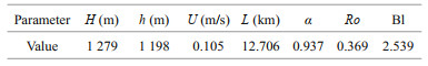
Several characteristic parameters like the fractional height of seamounts (α=h/H), the Rossby number (Ro=U/fL), and the blocking factor (Bl=α/Ro) have been put forward to determine whether a Taylor cap can form over a seamount. Here, h is the height of the seamount within the range of the impacting flow, H is the fluid depth, f is the Coriolis parameter, U is the average velocity of the impinging flow, and L is the horizontal length of the seamount (Hogg, 1973; Owens and Hogg, 1980; Chapman and Haidvogel, 1992; White et al., 2007).
The environmental conditions of the Y3 seamount and calculation results are given in Table 1. Different threshold values for the formation of Taylor caps have been determined in different works. The most popular value was put forward by Chapman and Haidvogel (1992). They proposed that the threshold value of Bl was 4 when α > 0.7; that is, the Taylor cap would form under the condition of Bl > 4. Additionally, they proposed that the Taylor cap would not form when the value of Ro was larger than 0.2. The calculation results showed that the value of Bl was 2.539 and the Ro of the Y3 seamount was 0.369 during the survey time, and neither value met the threshold values. It was difficult to form a Taylor cap under the above conditions. However, the velocity of the impinging flow at the Y3 seamount varied with time (Fig. 3), which meant that Ro and Bl also changed constantly. Therefore, a Taylor cap might form in the Y3 seamount, but it would not be a stable Taylor cap.
|
In addition to the Taylor cap, tides have also been found to induce the anticyclonic circulation over seamounts in many cases in previous studies (Eriksen, 1991; Kunze and Toole, 1997). Tidal currents over a seamount could generate the residual mean current, which is commonly referred to as tidal rectification. Tidal rectification results from the interaction of tidal currents and steep seabed, and the asymmetric tidal transport is caused by a combined impact of topographic acceleration and bottom friction. As a result, a cold dome which is similar to the uplifted isotherms generated by a Taylor cap forms over the seamount (Lavelle and Mohn, 2010).
In other words, the cold dome over the Y3 seamount could also be caused by tidal rectification. The contribution of tidal rectification can be evaluated, and it is instrumental in understanding the cause of the cold dome over a realistic seamount. Wright and Loder (1985) estimated the maximum residual flow that may arise under the most favorable conditions from the rectification of tidal currents as follows:
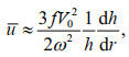 (1)
(1)where f is the local Coriolis parameter, h is the local depth, V0 is the amplitude of the tidal forcing, ω is the angular frequency of the tidal forcing, and dh/dr is the slope gradient. Utilizing the largest (1/h)·(dh/dr) at station Y3-11, h was 451 m, and dh/dr was 0.344 rad. The estimated residual velocity was ~0.778 cm/s, which was the theoretical maximum residual current at station Y3-11 induced by tidal rectification; however, the realistic velocity of station Y3-11 might be ~30 cm/s according to the flow velocity obtained by ADCP. The reason why tidal rectification had little contribution to the cold dome of the Y3 seamount was probably due to the weak bottom friction caused by the gradual slope of the seamount.
Since the Taylor cap could not form during the survey time and the contribution of tidal rectification was negligible, the cold dome over the top of the Y3 seamount was probably caused by upwelling. When the mean current encounters the seamount, the current climbs up with rough topography and carries the deep cold water upward, resulting in the formation of a cold dome above the summit. Upwelling is a relatively common phenomenon in steep topographies, and it forms more easily than a Taylor cap or tidal rectification.
3.2.3 Distribution of turbulent diffusivities and their influencing factorsTurbulent mixing can cause the transfer of momentum, heat, and matter in the horizontal and vertical directions. To maintain stabilization of ocean stratification, Munk (1966) put forward that the average turbulent diffusivity should reach at least 10-4 m2/s. However, the turbulent diffusivities were only 10-6–10-5 m2/s in the open ocean previously studied (Gregg, 1987; Ledwell et al., 1993; Kunze and Sanford, 1996). Thus, some people considered that diapycnal mixing may be enhanced near rough topographies. Studies in the last three decades have found much stronger turbulent mixing over ridges, seamounts, canyons, and hydraulically controlled passages (Lueck and Mudge, 1997; Ferron et al., 1998; Carter and Gregg, 2002; Klymak et al., 2006). As a consequence, the average turbulent diffusivity of the world's ocean was still likely up to 10-4 m2/s. As mentioned above, these special areas have a significant influence on the transfer of matter and heat in the world's ocean.
The Thorpe scale method based on the potential temperature (with noise of 0.001 ℃) was used to calculate the turbulent diffusivity (K) in the Y3 seamount (Ferron et al., 1998). The resolvable Thorpe scale depends on the sampling frequency of the potential temperature and the sampling instrument noise level. We used CTD data which were previously quality controlled, filtered, and subsampled to 1-m intervals to reduce high-frequency noise in this work. Therefore, we could not resolve gravitational overturns shorter than 2 m or Thorpe scales smaller than 1 m. It is sufficient to resolve the main instabilities using the CTD dataset, but Thorpe scales those were equal to 0 do not mean that there must be no overturn. The K profiles of all 13 stations are shown in Figs. 11 & 12. The high K values at the Y3 seamount were mostly distributed in the surface layer and near the bottom, with magnitudes of 10-4–10-1 m2/s (Figs. 11b, 12b). In the following, the main influencing factors of the high K values in the surface layer and near the bottom are discussed respectively.

|
| Fig.11 Vertical distribution of the turbulent diffusivities in Section NE of the Y3 seamount a. 0–300 m of Section NE; b. 0–2 000 m of Section NE. |

|
| Fig.12 Vertical distribution of the turbulent diffusivities in Section NW of the Y3 seamount a. 0-300 m of Section NW; b. 0-3 000 m of Section NW. |
Tides, surface wind stress, and mesoscale eddies are the main factors affecting the mixing of the surface layer (Richardson et al., 2000; Lavelle et al., 2004; Muench et al., 2009).
The thicknesses of the surface turbulent layers at different stations were different (Figs. 11a & 12a). Previous studies have shown that there was a certain correlation between turbulence and tidal phase (Muench et al., 2009; Padman et al., 2009). The tide heights at the Y3 seamount in December 2014 were extracted by TMD. The spring-neap tidal cycle was obvious during this month (Fig. 13). At the same time, the connection between the thickness of the surface turbulent layer and the spring-neap tidal cycle was significant. Stations with thicknesses of surface turbulent layers less than 40 m were investigated during neap tide, and stations with thicknesses greater than 50 m were investigated during spring tide. We further analyzed the correlation between the thickness of the surface turbulent layer and the four main tidal constituents of the Y3 seamount (Fig. 14). The results showed that there were moderate connections between the thickness of the surface turbulent layer and constituents M2, S2, and K1, while the correlation between the thickness and diurnal constituent O1 was weak. Semidiurnal constituents had a more significant effect on the surface turbulence in the Y3 seamount than diurnal constituents. The larger the tidal velocity was, the thicker the surface turbulent layer was.

|
| Fig.13 Tide height at the Y3 seamount in December 2014S These data were got from TPXO global, regional, and local tide models established by Oregon State University (Egbert and Erofeeva, 2002). Stations Y3-4, Y3-5, Y3-6, Y3-7, Y3-8, and Y3-9 were investigated from December 13 to 16, 2014 (blue shadow). Stations Y3-0, Y3-1, Y3-2, Y3-3, Y3-11, Y3-12, and Y3-13 were investigated from December 19 to 23, 2014 (orange shadow). |

|
| Fig.14 Correlations between the thickness of the surface turbulent layer and four main tidal constituents of the Y3 seamount These data were got from TPXO local and regional (Egbert and Erofeeva, 2002). The blue dots represent the stations investigated during neap tide, and the orange dots represent the stations investigated during spring tide. |
Second, the turbulent diffusivity at the surface layer is always affected by surface wind stress. The wind stress can be calculated based on wind field data using the conventional equation as follows (Pickett and Paduan, 2003):
 (2)
(2)where ρa is the density of air (we took a value of 1.173 kg/m3 since the air temperature was 28 ℃ during the investigation), U10 is the wind vector at 10 m above the sea surface, and the drag coefficient Cd can be defined as (under any wind speed and sea air temperature difference) (Ji et al., 2013):
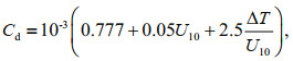 (3)
(3)where ΔT is the air-sea temperature difference.
Under pure wind stress forcing, the rate of dissipation of kinetic energy is defined as follows (Oakey, 1985; Yamazaki and Kamykowski, 1991):
 (4)
(4)where κ=0.4 is von Karman's constant, z is the vertical coordinate, and the friction velocity u* is defined by
 (5)
(5)where ρw is the water density. It can be deduced from Eqs.4 and 5 that the relationship between the rate of dissipation of kinetic energy and the wind stress is
 (6)
(6)Moreover, the turbulent diffusivity (K) is defined by
 (7)
(7)where Γ is the mixing efficiency and represents the ratio of the turbulent kinetic energy (TKE) converted into potential energy to the dissipated TKE. The mixing efficiency is generally 0.2. In addition, N is the buoyancy frequency. Equations 6 and 7 can now be used to relate the turbulent diffusivity measurements to wind stress. The monthly average wind speed at the height of 10 m above the ocean surface around the Y3 seamount in December 2014 is shown in Fig. 15. The wind speed around the Y3 seamount was relatively high in December 2014 and the maximum wind speed was 11.443 m/s during the survey time. As a result, the magnitudes of the turbulent diffusivities caused by surface wind stress were between 10-3–10-2 m2/s in the surface layers of the Y3 seamount. The surface wind stress greatly influenced the turbulent mixing of the Y3 seamount.

|
| Fig.15 The monthly mean wind field at 10 m above the sea surface around the Y3 seamount in December 2014 The monthly mean wind data were calculated from the daily ERA-Interim Reanalysis data provided by the ECMWF from their website at https://www.ecmwf.int/. The black triangle represents the Y3 seamount. |
Furthermore, the influence of the eddy was also taken into account. Seamounts are thought to be where eddies generate and destruct, so eddies are bound to have an effect on the dynamic environment of seamounts (Royer, 1978; Herbette et al., 2003). Distribution of SSHA around the study area in December 2014 is shown in Fig. 16. Both warm and cold eddies were present in the study area, and the activities of these eddies were energetic. Specifically, there was a very weak warm eddy east of the Y3 seamount on December 10 (Fig. 16a). This eddy moved westward and enhanced gradually with time, and then, it was obstructed by the topography when passing through the Yap Arc (Fig. 16c & d). Hydrodynamic models and observations suggest that during collisions with seamounts, eddies may be trapped and then disintegrate over the seamount, split or just rotate around the seamount. However, even eddies survive the collision, they may transfer their own water and energy to the seamount system (Richardson et al., 2000; Adduce and Cenedese, 2004). This energy can be used to produce turbulence in seamounts. The high values of K in the Y3 seamount may be in part related to the activities of these eddies.

|
| Fig.16 SSHA around the Y3 seamount during the survey 16:20:17 a. December 10; b. December 15; c. December 20; d. December 25. The black triangle represents the Y3 seamount. |
Previous studies have shown that the interaction between semidiurnal tides and topography will generate the most energetic internal tides. Therefore, the intensity of internal tides on the steep slopes and summit of a seamount is relatively high (Munk, 1981; Lavelle and Mohn, 2010). Noble et al. (1988) deployed a current meter continuously for 9 months above Horizon Guyot. The large isotherm deflections, large M2 current amplitude, and current-temperature phase relationships all proved that the semidiurnal tides over Horizon Guyot were predominantly baroclinic (internal tides). They thought that semidiurnal internal tides were generated at the guyot since the observed tidal characteristics did not correspond to those of an internal tide observed far from a generation region. Noble and Mullineaux (1989) found that the semidiurnal currents over the Cross seamount were due to baroclinic (internal) tides rather than to barotropic tides, and the internal tides were likely generated at the ridge of seamounts 100 km to the east of the Cross seamount. Numerical investigations and laboratory experiments were also conducted to study the internal tides over a seamount (Holloway and Merrifield, 1999; Wang et al., 2017).
Near the bottom of the Y3 seamount, turbulent diffusivities were different in the two sections. The turbulence near the bottom of Section NE was stronger than that of Section NW (Figs. 11b & 12b). The turbulent diffusivities were higher around the rougher bottom (Fig. 11b) and vice versa (Fig. 12b). Generally, the Y3 seamount can also produce internal tides. Once the internal tides break, their energy will be redistributed, resulting in energetic turbulent mixing (Rudnick et al., 2003; van Haren and Gostiaux, 2012). The distribution of turbulent diffusivities near the bottom of the Y3 seamount is in good agreement with this dynamic mechanism. Therefore, the interaction between topography and tides was possibly the cause of the turbulent mixing near the bottom of the Y3 seamount. Besides, the interaction of topography and the bottom currents may also cause intense turbulent mixing near the bottom of the Y3 seamount, and to confirm this hypothesis, current measurement near the bottom is necessary.
In summary, tides and surface wind stress, particularly the interaction between the Y3 seamount and mesoscale eddies and all kinds of currents, could all be crucial factors influencing the distribution of turbulent diffusivities at the Y3 seamount. Furthermore, the high turbulent diffusivities of the Y3 seamount (especially the high values at the bottom) showed that these special areas did have a great impact on the global mean turbulent diffusivity.
4 CONCLUSIONIn the winter of 2014, the upper layer (150 m) of the Y3 seamount was dominated by the westward-flowing NEC with a comparatively large velocity of 0.10–0.40 m/s. The water between 200–800 m was dominated by the eastward-flowing NEUC, which had a low velocity, 0.03–0.20 m/s. The Y3 seamount played an important role in the current distribution. The current direction below 550 m changed to the completely opposite direction as the NEUC jet at upstream station Y3-9. At station Y3-11 on the leeward side, the flow direction below 300 m fluctuated greatly. The flow directions below 300 m of station Y3-12 on the leeward side were westward. These were likely caused by the Y3 seamount obstacle for the NEUC, or they may have been related to temporal variations.
An obvious surface mixed layer existed during the survey time, and its depth was ~50 m. The water column was intensively stratified between ~50– 150 m. The NPTW with high salinity was distributed in the subsurface layer of the Y3 seamount, and the uneven distribution of salinity in the middle layer resulted from the mixing of AAIW and NPIW. The calculations indicated that the cold dome over the Y3 seamount was not caused by a Taylor cap or tidal rectification, and it was probably caused by upwelling.
The high turbulent diffusivities with magnitudes of 10-4–10-1 m2/s in the Y3 seamount were almost distributed in the surface layers and near bottom layers. In the surface layer, the thicknesses of the turbulent layers were greatly influenced by the spring-neap tidal cycle, and the influence of semidiurnal constituents was greater than that of diurnal constituents. A calculation result showed that the surface wind stress greatly affected the turbulent mixing of the Y3 seamount, but the correlation between the high surface turbulent diffusivities and activities of eddies was weak. Near the bottom of the Y3 seamount, the interaction of the rough topography and semidiurnal tides was the most likely cause of internal tides, which then led to turbulent mixing and high turbulent diffusivities at most stations. The turbulent diffusivities were higher in the rougher bottom layer and vice versa. In addition, the interaction of topography and the bottom currents may also cause intense turbulent mixing near the bottom.
5 DATA AVAILABILITY STATEMENTThe field survey datasets supporting the current work are available from the corresponding author on reasonable request. All of the links of open-access datasets are included in this article.
6 ACKNOWLEDGMENTWe thank the captain, crew, and scientists of R/V Kexue for their great efforts. We also thank the reviewers for their perceptive suggestions.
Adduce C, Cenedese C. 2004. An experimental study of a mesoscale vortex colliding with topography of varying geometry in a rotating fluid. Journal of Marine Research, 62(5): 611-638.
DOI:10.1357/0022240042387583 |
Bashmachnikov I, Loureiro C M, Martins A. 2013. Topographically induced circulation patterns and mixing over Condor seamount. Deep Sea Research Part II: Topical Studies in Oceanography, 98: 38-51.
DOI:10.1016/j.dsr2.2013.09.014 |
Bosc C, Delcroix T, Maes C. 2009. Barrier layer variability in the western Pacific warm pool from 2000 to 2007. Journal of Geophysical Research: Oceans, 114(C6): C06023.
DOI:10.1029/2008JC005187 |
Brink K H. 1995. Tidal and lower frequency currents above Fieberling Guyot. Journal of Geophysical Research: Oceans, 100(C6): 10817-10832.
DOI:10.1029/95JC00998 |
Carter G S, Gregg M C. 2002. Intense, variable mixing near the head of Monterey submarine canyon. Journal of Physical Oceanography, 32(11): 3145-3165.
DOI:10.1175/1520-0485(2002)032<3145:IVMNTH>2.0.CO;2 |
Chapman D C, Haidvogel D B. 1992. Formation of Taylor caps over a tall isolated seamount in a stratified ocean. Geophysical & Astrophysical Fluid Dynamics, 64(1-4): 31-65.
DOI:10.1080/03091929208228084 |
Chassignet E P, Hurlburt H E, Smedstad O M, Halliwell G R, Hogan P J, Wallcraft A J, Bleck R. 2006. Ocean prediction with the hybrid coordinate ocean model (HYCOM). In: Chassignet E P, Verron J eds. Ocean Weather Forecasting: an Integrated View of Oceanography. Springer, Dordrecht. p. 413-426.
|
Dai S, Zhao Y F, Li X G, Wang Z Y, Zhu M L, Liang J H, Liu H J, Tian Z Y, Sun X X. 2020. The seamount effect on phytoplankton in the tropical western Pacific. Marine Environmental Research, 162: 105094.
DOI:10.1016/j.marenvres.2020.105094 |
Dower J, Freeland H, Juniper K. 1992. A strong biological response to oceanic flow past Cobb Seamount. Deep Sea Research Part A. Oceanographic Research Papers, 39(7-8): 1139-1145.
DOI:10.1016/0198-0149(92)90061-W |
Egbert G D, Erofeeva S Y. 2002. Efficient inverse modeling of barotropic ocean tides. Journal of Atmospheric and Oceanic Technology, 19(2): 183-204.
DOI:10.1175/1520-0426(2002)019<0183:EIMOBO>2.0.CO;2 |
Eriksen C C. 1991. Observations of amplified flows atop a large seamount. Journal of Geophysical Research: Oceans, 96(C8): 15227-15236.
DOI:10.1029/91jc01176 |
Ferron B, Mercier H, Speer K, Gargett A, Polzin K. 1998. Mixing in the romanche fracture zone. Journal of Physical Oceanography, 28(10): 1929-1945.
DOI:10.1175/1520-0485(1998)028<1929:mitrfz>2.0.co;2 |
Fine R A, Lukas R, Bingham F M, Warner M J, Gammon R H. 1994. The western equatorial Pacific: a water mass crossroads. Journal of Geophysical Research: Oceans, 99(C12): 25063-25080.
DOI:10.1029/94JC02277 |
Genin A, Dayton P K, Lonsdale P F, Spiess F N. 1986. Corals on seamount peaks provide evidence of current acceleration over deep-sea topography. Nature, 322(6074): 59-61.
DOI:10.1038/322059a0 |
Genin A, Dower J F. 2007. Seamount plankton dynamics. In: Pitcher T J, Morato T, Hart P J B, Clark M R, Haggan N, Santos R S eds. Seamounts: Ecology, Fisheries & Conservation. Blackwell Publishing, Hoboken. p. 85-100, https://doi.org/10.1002/9780470691953.
|
Genin A. 2004. Bio-physical coupling in the formation of zooplankton and fish aggregations over abrupt topographies. Journal of Marine Systems, 50(1-2): 3-20.
DOI:10.1016/J.Marsys.2003.10.008 |
Gregg M C. 1987. Diapycnal mixing in the thermocline: a review. Journal of Geophysical Research: Oceans, 92(C5): 5249-5286.
DOI:10.1029/JC092iC05p05249 |
Guo B B, Wang W Q, Shu Y Q, He G W, Zhang D S, Deng X G, Liang Q Y, Yang Y, Xie Q, Wang H F, Wang J. 2020. Observed deep anticyclonic cap over Caiwei Guyot. Journal of Geophysical Research: Oceans, 125(10): e2020JC016254.
DOI:10.1029/2020JC016254 |
Herbette S, Morel Y, Arhan M. 2003. Erosion of a surface vortex by a seamount. Journal of Physical Oceanography, 33(8): 1664-1679.
DOI:10.1175/2382.1 |
Hogg N G. 1973. On the stratified Taylor column. Journal of Fluid Mechanics, 58(3): 517-537.
DOI:10.1017/S0022112073002302 |
Holloway P E, Merrifield M A. 1999. Internal tide generation by seamounts, ridges, and islands. Journal of Geophysical Research: Oceans, 104(C11): 25937-25951.
DOI:10.1029/1999jc900207 |
Hu D X, Cui M C. 1991. The western boundary current of the Pacific and its role in the climate. Chinese Journal of Oceanology and Limnology, 9(1): 1-14.
DOI:10.1007/BF02849784 |
Hu D X, Wu L X, Cai W J, Gupta A S, Ganachaud A, Qiu B, Gordon A L, Lin X P, Chen Z H, Hu S J, Wang G J, Wang Q Y, Sprintall J, Qu T D, Kashino Y, Wang F, Kessler W S. 2015. Pacific western boundary currents and their roles in climate. Nature, 522(7556): 299-308.
DOI:10.1038/nature14504 |
Ji W J, Zhang S W, Zhao H, Cao R X, Cheng Y H, Xie L L. 2013. Impact of the sea surface coefficient CD to the air-sea temperature difference. Marine Forecasts, 30(5): 63-68.
(in Chinese with English abstract) DOI:10.11737/j.issn.1003-0239.2013.05.010 |
Klymak J M, Moum J N, Nash J D, Kunze E, Girton J B, Carter G S, Lee C M, Sanford T B, Gregg M C. 2006. An estimate of tidal energy lost to turbulence at the Hawaiian Ridge. Journal of Physical Oceanography, 36(6): 1148-1164.
DOI:10.1175/JPO2885.1 |
Kunze E, Sanford T B. 1996. Abyssal mixing: where it is not. Journal of Physical Oceanography, 26(10): 2286-2296.
DOI:10.1175/1520-0485(1996)026<2286:AMWIIN>2.0.CO;2 |
Kunze E, Toole J M. 1997. Tidally driven vorticity, diurnal shear, and turbulence atop fieberling seamount. Journal of Physical Oceanography, 27(12): 2663-2693.
DOI:10.1175/1520-0485(1997)027<2663:TDVDSA>2.0.CO;2 |
Lavelle J W, Lozovatsky I D, Smith IV D C. 2004. Tidally induced turbulent mixing at Irving Seamount—modeling and measurements. Geophysical Research Letters, 31(10): L10308-10.1029/2004GL019706.
DOI:10.1029/2004GL019706 |
Lavelle J W, Mohn C. 2010. Motion, commotion, and biophysical connections at deep ocean seamounts. Oceanography, 23(1): 90-103.
DOI:10.5670/oceanog.2010.64 |
Ledwell J R, Watson A J, Law C S. 1993. Evidence for slow mixing across the pycnocline from an open-ocean tracerrelease experiment. Nature, 364(6439): 701-703.
DOI:10.1038/364701a0 |
Levine A F Z, McPhaden M J. 2016. How the July 2014 easterly wind burst gave the 2015-2016 El Niño a head start. Geophysical Research Letters, 43(12): 6503-6510.
DOI:10.1002/2016GL069204 |
Li F Q, Su Y S. 2000. Analysis of Water Masses in Oceans. Qingdao Ocean University Press, Qingdao, China. 397p. (in Chinese)
|
Lian T, Chen D K, Tang Y M. 2017. Genesis of the 2014-2016 El Niño events. Science China Earth Sciences, 60(9): 1589-1600.
DOI:10.1007/s11430-016-8315-5 |
Lueck R G, Mudge T D. 1997. Topographically induced mixing around a shallow seamount. Science, 276(5320): 1831-1833.
DOI:10.1126/science.276.5320.1831 |
Lukas R, Lindstrom E. 1991. The mixed layer of the western equatorial Pacific Ocean. Journal of Geophysical Research: Oceans, 96(S01): 3343-3357.
DOI:10.1029/90JC01951 |
Maes C, Ando K, Delcroix T, Kessler W S, McPhaden M J, Roemmich D. 2006. Observed correlation of surface salinity, temperature and barrier layer at the eastern edge of the western Pacific warm pool. Geophysical Research Letters, 33(6): L06601.
DOI:10.1029/2005GL024772 |
Masumoto Y, Yamagata T. 1991. Response of the western tropical Pacific to the Asian winter monsoon: the generation of the Mindanao dome. Journal of Physical Oceanography, 21(9): 1386-1398.
DOI:10.1175/1520-0485(1991)021<1386:ROTWTP>2.0.CO;2 |
Mohn C, Beckmann A. 2002. The upper ocean circulation at Great Meteor Seamount. Ocean Dynamics, 52(4): 179-193.
DOI:10.1007/s10236-002-0017-4 |
Muench R, Padman L, Gordon A, Orsi A. 2009. A dense water outflow from the Ross Sea, Antarctica: mixing and the contribution of tides. Journal of Marine Systems, 77(4): 369-387.
DOI:10.1016/j.jmarsys.2008.11.003 |
Munk W H. 1966. Abyssal recipes. Deep Sea Research and Oceanographic Abstracts, 13(4): 707-730.
DOI:10.1016/0011-7471(66)90602-4 |
Munk W H. 1981. Internal waves and small-scale processes. In: Warren B A, Wunsch C eds. Evolution of Physical Oceanography. MIT Press, Cambridge. p. 264-276.
|
Noble M, Cacchione D A, Schwab W C. 1988. Observations of strong mid-pacific internal tides above horizon guyot. Journal of Physical Oceanography, 18(9): 1300-1306.
DOI:10.1175/1520-0485(1988)018<1300:OOSMPI>2.0.CO;2 |
Noble M, Mullineaux L S. 1989. Internal tidal currents over the summit of cross seamount. Deep Sea Research Part A. Oceanographic Research Papers, 36(12): 1791-1802.
DOI:10.1016/0198-0149(89)90112-X |
Oakey N S. 1985. Statistics of mixing parameters in the upper ocean during JASIN Phase 2. Journal of Physical Oceanography, 15(12): 1662-1675.
DOI:10.1175/1520-0485(1985)015<1662:SOMPIT>2.0.CO;2 |
Owens W B, Hogg N G. 1980. Oceanic observations of stratified Taylor columns near a bump. Deep Sea Research Part A. Oceanographic Research Papers, 27(12): 1029-1045.
DOI:10.1016/0198-0149(80)90063-1 |
Padman L, Howard S L, Orsi A H, Muench R D. 2009. Tides of the northwestern Ross Sea and their impact on dense outflows of Antarctic Bottom Water. Deep Sea Research Part II: Topical Studies in Oceanography, 56(13-14): 818-834.
DOI:10.1016/j.dsr2.2008.10.026 |
Pickett M H, Paduan J D. 2003. Ekman transport and pumping in the California Current based on the U.S. Navy's highresolution atmospheric model (COAMPS). Journal of Geophysical Research, 108(C10): 3327.
DOI:10.1029/2003JC001902 |
Qiu B, Rudnick D L, Chen S M, Kashino Y. 2013. Quasi-stationary North Equatorial Undercurrent jets across the tropical North Pacific Ocean. Geophysical Research Letters, 40(10): 2183-2187.
DOI:10.1002/grl.50394 |
Read J, Pollard R. 2017. An introduction to the physical oceanography of six seamounts in the southwest Indian Ocean. Deep Sea Research Part II: Topical Studies in Oceanography, 136: 44-58.
DOI:10.1016/j.dsr2.2015.06.022 |
Richardson P L, Bower A S, Zenk W. 2000. A census of Meddies tracked by floats. Progress in Oceanography, 45(2): 209-250.
DOI:10.1016/S0079-6611(99)00053-1 |
Roden G I, Taft B A. 1985. Effect of the Emperor Seamounts on the mesoscale thermohaline structure during the summer of 1982. Journal of Geophysical Research: Oceans, 90(C1): 839-855.
DOI:10.1029/JC090iC01p00839 |
Roden G I. 1994. Effects of the Fieberling seamount group upon flow and thermohaline structure in the spring of 1991. Journal of Geophysical Research: Oceans, 99(C5): 9941-9961.
DOI:10.1029/94JC00057 |
Royer T C. 1978. Ocean eddies generated by seamounts in the North Pacific. Science, 199(4333): 1063-1064.
DOI:10.1126/science.199.4333.1063-a |
Rudnick D L, Boyd T J, Brainard R E, Carter G S, Egbert G D, Gregg M C, Holloway P E, Klymak J M, Kunze E, Lee C M, Levine M D, Luther D S, Martin J P, Merrifield M A, Moum J N, Nash J D, Pinkel R, Rainville L, Sanford T B. 2003. From tides to mixing along the Hawaiian ridge. Science, 301(5631): 355-357.
DOI:10.1126/science.1085837 |
Shi X Y, Wang Z Y, Huang H J. 2021. Physical oceanography of the Caroline M4 seamount in the tropical western Pacific Ocean in summer 2017. Journal of Oceanology and Limnology, 39(5): 1634-1650.
DOI:10.1007/s00343-021-0359-8 |
Sprintall J, Tomczak M. 1992. Evidence of the barrier layer in the surface layer of the tropics. Journal of Geophysical Research: Oceans, 97(C5): 7305-7316.
DOI:10.1029/92JC00407 |
van Haren H, Gostiaux L. 2012. Detailed internal wave mixing above a deep-ocean slope. Journal of Marine Research, 70(1): 173-197.
DOI:10.1357/002224012800502363 |
Wallcraft A J, Kara A B, Barron C N, Metzger E J, Pauley R L, Bourassa M A. 2009. Comparisons of monthly mean 10 m wind speeds from satellites and NWP products over the global ocean. Journal of Geophysical Research: Atmospheres, 114(D16): D16109.
DOI:10.1029/2008JD011696 |
Wang F J, Feng J Q, Wang Q Y, Zhang L L, Hu S J, Hu D X. 2020. Instability in boundary layer between the North Equatorial Current and underlying zonal jets based on mooring observations. Journal of Oceanology and Limnology, 38(5): 1368-1381.
DOI:10.1007/s00343-020-0015-8 |
Wang F, Zang N, Li Y L, Hu D X. 2015. On the subsurface countercurrents in the Philippine Sea. Journal of Geophysical Research: Oceans, 120(1): 131-144.
DOI:10.1002/2013JC009690 |
Wang J H, Wang S Y, Chen X, Wang W, Xu Y. 2017. Three-dimensional evolution of internal waves reflected from a submarine seamount. Physics of Fluids, 29(10): 106601.
DOI:10.1063/1.4986167 |
White M, Bashmachnikov I, Arístegui J, Martins A. 2007. Physical processes and seamount productivity. In: Pitcher T J, Morato T, Hart P J B, Clark M R, Haggan N, Santos R S eds. Seamounts: Ecology, Fisheries & Conservation. Blackwell Publishing, Hoboken. p. 65-84, https://doi.org/10.1002/9780470691953.ch4.
|
Wright D G, Loder J W. 1985. A depth-dependent study of the topographic rectification of tidal currents. Geophysical & Astrophysical Fluid Dynamics, 31(3-4): 169-220.
DOI:10.1080/03091928508219269 |
Xie L L, Tian J W, Hu D X, Wang F. 2009. A quasi-synoptic interpretation of water mass distribution and circulation in the western North Pacific: I. Water mass distribution. Chinese Journal of Oceanology and Limnology, 27(3): 630-639.
DOI:10.1007/s00343-009-9161-8 |
Yamazaki H, Kamykowski D. 1991. The vertical trajectories of motile phytoplankton in a wind-mixed water column. Deep Sea Research Part A. Oceanographic Research Papers, 38(2): 219-241.
DOI:10.1016/01980149(91)90081-P |
Yesson C, Letessier T B, Nimmo-Smith A, Hosegood P, Brierley A S, Harouin M, Proud R. 2020. Improved bathymetry leads to 4000 new seamount predictions in the global ocean. UCL Open: Environment Preprint, https://doi.org/10.14324/111.444/000044.v1.
|
Zhang J L, Xu K D. 2013. Progress and prospects in seamount biodiversity. Advances in Earth Science, 28(11): 1209-1216.
(in Chinese with English abstract) |
Zhang L L, Wang F J, Wang Q Y, Hu S J, Wang F, Hu D X. 2017. Structure and variability of the North equatorial current/undercurrent from mooring measurements at 130°E in the western Pacific. Scientific Reports, 7: 46310.
DOI:10.1038/srep46310 |
Zhang Q L, Zhou H, Liu H W. 2012. Interannual variability in the Mindanao Eddy and its impact on thermohaline structure pattern. Acta Oceanologica Sinica, 31(6): 56-65.
DOI:10.1007/s13131-012-0247-3 |