 2022, Vol. 40
Institute of Oceanology, Chinese Academy of Sciences
Article Information
- HAN Bing
- The energy conversion rates from eddies and mean flow into internal lee waves in the global ocean
- Journal of Oceanology and Limnology, 40(4): 1304-1313
- http://dx.doi.org/10.1007/s00343-021-1085-y
Article History
- Received Mar. 15, 2021
- accepted in principle Jun. 16, 2021
- accepted for publication Aug. 18, 2021


2 State Key Laboratory of Tropical Oceanography, South China Sea Institute of Oceanology, Chinese Academy of Sciences, Guangzhou 510301, China;
3 Institut für Meereskunde, Universität Hamburg, Hamburg 20146, Germany;
4 Key Laboratory of Climate, Resources and Environment in Continental Shelf Sea and Deep Sea of Department of Education of Guangdong Province, Guangdong Ocean University, Zhanjiang 524088, China
The meridional overturning circulation (MOC) transports and redistributes mass, heat, salt, CO2, and nutrients around the globe, and has an important influence on the climate. Diapycnal mixing caused by wave breaking and other processes can bring the deep water to the ocean surface and plays a crucial role in sustaining the MOC. About 2 TW is needed for diapycnal mixing in the global ocean (Munk and Wunsch, 1998). The energy mainly comes from three types of motions: the near-inertial waves generated by winds in upper ocean, the internal tides generated by barotropic tides over bottom topography, and internal lee waves generated by geostrophic flows over bottom topography (Egbert and Ray, 2001; Alford, 2003; Garabato et al., 2004; Brearley et al., 2013; Rimac et al., 2013; Liu et al., 2019).
Mesoscale eddies are the largest kinetic energy reservoir in the global ocean, which can transport tracers and regulate global climate change (Ferrari and Wunsch, 2009). Eddies can be generated by barotropic and baroclinic instability, and dissipate through several processes. For example, they can dissipate through the bottom dissipation (Sen et al., 2008; Arbic et al., 2009), loss of balance (Molemaker et al., 2005; Polzin, 2010; Shakespeare and Taylor, 2013, 2014, 2015; Shakespeare, 2019), interactions with other motions (Polzin, 2008; Zhang et al., 2020), generation of submesoscale motions and internal lee waves (Trossman et al., 2013; Melet et al., 2014; Trossman et al., 2015, 2016; Kunze, 2019; Yang at al., 2019). However, how much eddy energy dissipates through different mechanisms remains poorly understood. Recently, the total energy flux into internal lee waves from geostrophic flow has been estimated and found to be about 0.2–0.94 TW based on linear theory (Nikurashin and Ferrari, 2011; Scott et al., 2011; Wright et al., 2014). In addition, Yang et al. (2018) estimated the energy loss of eddies due to lee wave generation (0.12 TW) in the Southern Ocean. However, the difference in energy conversion between from eddies and from the mean flow in the global ocean remains unclear.
Previous research has investigated the turbulent dissipation in the South Ocean, and found large difference between the observed dissipation rate and theoretical prediction of energy conversion rate of lee waves (Sheen et al., 2013; Waterman et al., 2013, 2014; Cusack et al., 2017). For example, Waterman et al. (2013) showed that the conversion rate estimated by the linear theory (Nikurashin and Ferrari, 2011) was much larger than the observed dissipation rate in a region north of the Kerguelen Pkateau. These differences can be explained in many ways; for example, much of the energy may propagate away from the generation sites (Zheng and Nikurashin, 2019), the linear theory may ignore some finite topography effects (Nikurashin et al., 2014), and there are limitations for the topographic spectrum (Nikurashin et al., 2014). Motivated by the difference between the observed dissipation rate and the energy conversion rate estimated by linear theory, the paper investigates whether different data processing procedures on calculating the topographic spectra and topographic data resolution can have an important influence on the estimated global energy conversion, which has not been well investigated so far. In this study, new methods were developed to compute the energy conversion. Results show that the above-mentioned factors could cause inaccuracies on the calculation of energy conversion in the global ocean.
This article is arranged as follows: in Section 2, the data and methods used for calculations are described; in Section 3, the energy conversion rates from the mean flow and eddies are computed; in Section 4, the uncertainties of energy conversion caused by dealing with the topographic data are discussed; The conclusions are shown in Section 5.
2 DATA AND METHOD 2.1 TheoryThe energy flux transferred from geostrophic flows to internal lee waves in small-cale topography is given by (Bell, 1975; Nikurashin and Ferrari, 2011; Nikurashin et al., 2014),
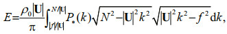 (1)
(1)where the reference density ρ0=1 045 kg/m3, U is the bottom velocity, N is the bottom stratification, f is the Coriolis frequency and 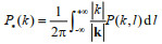
To calculate the energy generation rate of lee waves from eddies and mean flow, the full velocity is divided into the time-mean flow and eddy velocity and the results are obtained by using Eq.1. This method is different from the former research (Yang et al., 2018) in which they divided both the velocity and lee wave drag into their time-mean and transient components. They then calculated the energy loss from eddies and mean flow due to lee wave generation.
The generation of lee waves is largely influenced by the steepness parameter ε=NH/|U| (Nikurashin and Ferrari, 2010a, 2010b, 2011; Nikurashin et al., 2014), where 
The key quantities in this calculation are the topographic spectra, topographic height, bottom stratification, and bottom velocity, which will be introduced in the next sections.
2.2 Topographic spectraFollowing the method of Goff and Jordan (1998) and Nikurashin and Ferrari (2011), and assuming the topography is isotropic, the effective topographic spectrum in Eq.1 then can be calculated by
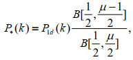 (2)
(2)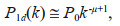 (3)
(3)where B is the Beta function, P1d(k) is a one-dimensional form of model spectrum, P0 is the spectral level given in terms of parameters of the two-dimensional spectrum and μ is the spectral slope.
Here, P1d(k) is computed using single beam sounding from U.S. National Geophysical Data Center's Marine Trackline Geophysics database. The database provides access to bathymetry data collected during marine cruises from 1939 to the present and its coverage is worldwide. Data sources include global oceanographic institutions, universities, and government agencies. The resolution of the data in the Southern Ocean is smaller than that in the Northern Ocean.
The topographic spectra are estimated as follows. The single beam sounding depth data deeper than 500 m is divided into different segments with a resolution of at least 2 km and a length of 50 km, the topographic slope is removed for each segment, then the along track topographic spectrum is calculated. Using Eq.3, P0 and μ are obtained in the 2 to 20 km wavelength range.
Due to the limitation of the spatial resolution of topographic data, the resolution of energy conversion rate is 3°×3°. There are two methods to calculate the energy conversion rate. The first method (hereinafter referred to as "RF") (Nikurashin and Ferrari, 2011) is introduced as follows. The topographic spectra of different segments over a 3°×3° grid are averaged, and P0 and μ are calculated in each grid. Then the conversion rate with a resolution of 3°×3° can be computed by using P0 and μ. Absent values due to lack of topographic data are estimated from neighboring grid cells.
In order to investigate whether different data processing procedures can have a large influence on the results even for the same topographic data, a new method is developed to compute the conversion rate. The second method (hereinafter referred to as "RS") is introduced as follows. Instead of averaging the topographic spectra over a 3°×3° grid, P0 and μ in each segment are calculated first; then P0 and μ are divided into 3°×3° grid cells. Using the bottom velocity U, stratification N, P0, and μ from a 3°×3° grid cell, the conversion rates can be obtained in each grid. Moreover, by using this method, the mean conversion rate can be got by averaging the rates over the same grid, and the largest and smallest conversion rates can also be obtained by setting the rate as the maximum and minimum value within the same grid. The total number of about 225 000 segments is used.
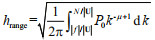
2.3 Topographic roughnessThe topographic roughness calculated from single beam soundings here is compared with the global abyssal hill rms heights (Goff and Arbic, 2010). The topographic roughness calculated from single beam soundings is defined in two ways.
The first way is H=hRF, where 
The second way is H=hRS, where 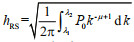
Following Goff and Arbic (2010), the global abyssal hill rms heights hrms are calculated using the paleo-spreading rate and sediment thickness by the following equation,
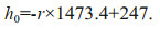 (4)
(4)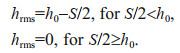 (5)
(5)where r is the spreading rate, h0 is the uncorrected rms height, and S is the sediment thickness (Eden and Olbers, 2014). The spreading rates of the world's ocean crust has a resolution of 2 min and covers all major ocean basins (Müller et al., 2008). The domain of NCEI's (National Centers for Environmental Information) global ocean sediment thickness extends from 60°E to 155°E, and 30°S to 70°S (Whittaker et al., 2013). The rms data has 1° spatial resolution. Only part of areas of ocean has hrms>0 using this method.
2.4 Bottom stratificationThe global bottom stratification is calculated by the World Ocean Circulation Experiment (WOCE) Global Hydrographic Climatology (Gouretski and Koltermann, 2004) which has a 0.5° spatial resolution and 45 depth levels. The potential pressure, potential temperature, and potential salinity from the bottom two layers are used for the calculation.
2.5 Bottom velocityThe bottom mean flow and eddy velocity are got from the global eddy-permitting STORM model (von Storch et al., 2012). The model was spun up for 25 years using the German Ocean Model Intercomparison Project (OMIP) forcing derived from the 15-year European Centre for Medium-Range Weather Forecasts (ECMWF) Re-Analysis (ERA-15). Then the model was run with the forcing of 6 hourly National Centers for Environmental Prediction (NCEP)-National Center for Atmospheric Research (NCAR) reanalysis-1 (Kalnay et al., 1996) for the period 1948–2010 with a resolution of about 1/10°, so it can achieve a quasi-steady state of mesoscale eddies. Further details of the model setup can be found in von Storch et al. (2012). Here the output of mean flow and eddy velocity are used, both of which have a resolution of 1°×1°.
The horizontal full velocity u=(u, v), the perturbation velocity u'=(u', v') and the mean flow Um=(U, V). The time-dependent eddy velocity is defined by u'(x, y, z, t)=u(x, y, z, t)–U(x, y, z). Where the mean flow can be obtained by 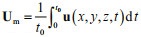
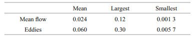
The mean flow kinetic energy is then obtained by MKE=U2+V2, while the eddy kinetic energy is defined by 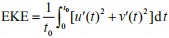

The values of bottom stratification N are between 10-3.5 s-1 and 10-2.5 s-1 over most of areas with high values of N in mid-ocean ridge and low values of N over abyssal ocean (Fig. 1). The values in the areas with a depth shallower than 500 m are not calculated.

|
| Fig.1 Bottom stratification N using the WOCE hydrographic atlas |
The bottom mean flow kinetic energy (MKE) and eddy kinetic energy (EKE) show a similar pattern that they are enhanced in Antarctic Circumpolar Current (ACC) region, west boundary currents and equatorial regions (Fig. 2). However, the EKE is larger than the MKE in most areas of the ocean, and its energy can be enhanced to 10-2 m2/s2 in ACC region, indicating the lee wave generation from eddies is larger than that from the mean flow.

|
| Fig.2 Bottom MKE (a) and bottom EKE (b) |
The topographic roughness calculated by using two kinds of data is compared (Fig. 3). The large hRF (Fig. 3a) is along mid-ocean ridges where the process of seafloor spreading occurs, and it is enhanced up to 100 m. The small roughness is in flat abyssal plains that are covered by sediments. hRS (Fig. 3b) shows a pattern similar to the Fig. 3a, though the roughness is a little smaller. It is up to 80 m along mid-ocean. The difference between hRF and hRS is caused by different calculation methods. In summary, most of areas of the ocean are covered with the topographic roughness of 0–100 m for hRF and hRS. The global abyssal hill rms heights hrms (Goff and Arbic, 2010) is shown in Fig. 3c. Compared with the hRF and hRS calculated from the single beam soundings, it has a similar pattern and can be enhanced to more than 200 m.

|
| Fig.3 Topographic roughness a. hRF; b. hRS; c. hrms. |
The steepness parameter is determined by the bottom buoyancy frequency, topographic height, and bottom velocity. The steepness parameters calculated using the mean flow and eddy velocity from the global eddy-permitting STORM model are shown in Fig. 4. The steepness parameter from the eddy velocity shows a pattern similar to that from the mean flow. In addition, it is also similar to the former results (Nikurashin and Ferrari, 2011). It is large in the areas with large bottom stratification or large topographic height, such as the equatorial regions and the mid-ocean ridges (Fig. 4), indicating the energy conversion in these areas should be corrected, while it is small in the ACC area because of large bottom current velocity.

|
| Fig.4 Topographic steepness parameter ε calculated using the mean flow (a) and eddy velocity (b) |
The importance of lee wave generation from eddies is compared with that from the mean flow. By using RF and topographic height hrange, the conversion rates from the mean flow and eddy velocity are calculated and shown in Fig. 5. The rates from the eddy velocity and mean flow are large in the large currents areas and show a pattern similar to the bottom kinetic energy, indicating that the bottom current velocity plays a crucial role in the lee wave generation. Though these spatial patterns are also similar to these obtained by previous studies (Nikurashin and Ferrari, 2011; Scott et al., 2011; Wright et al., 2014), the differences exist due to different bottom velocity data. The results also show that the rate from eddies is much larger than that from the mean flow, indicating that the lee wave generation is mainly from eddies instead of the mean flow. To better understand the difference in conversion rate between from eddies and from the mean flow, the rates are then integrated in the global ocean. Here the conversion rates in the areas with values larger than 2×10² mW/m2 are set to be 0 in order to inhibit large value. The energy conversion from the mean flow and eddies are 0.035 and 0.083 TW, respectively. Yang et al. (2018) pointed that the energy loss from eddies and mean flow due to lee wave generation in the Southern Ocean is 0.12 and 0.04 TW, respectively. The results that obtained in the paper are different from Yang et al. (2018) because different data have been used and calculations have been done using different methods and different velocity. However, both results highlight the importance of lee wave generation from eddies.

|
| Fig.5 Internal lee wave generation rate calculated from the mean flow (a) and eddies (b) |
As we know, the terrain is a crucial factor for generating internal lee waves. The previous studies have obtained different conversion rates by using different topographic data and the rate is also influenced by the anisotropy in small-scale topography (Scott et al., 2011; Yang et al., 2018). In this section, the goal is to prove that even for the same topographic data, different data processing procedures can obtain different results, and insufficient data resolution will cause inaccuracies in calculating the global energy conversion of lee waves.
To achieve the above goals, the smallest, mean, and largest conversion rate are calculated in the global ocean according to the method that is referred to the Section 2.2. The conversion rate computed by RF has been discussed before, hence the smallest, mean, and largest conversion rate by using RS are focused on in this section. The mean conversion rate has a similar meaning to the conversion rate obtained by RF. The meaning for the largest and smallest conversion rate is that the two values represent the upper and lower global integral energy conversion rates by using linear theory.
The mean conversion rate was compared with the rate obtained by RF. Figure 6b shows that the mean conversion rate is large in the ACC region, equatorial regions, and west boundary currents regions, and is similar to that obtained by RF. The integrated mean energy conversion from the mean flow and eddies in the global ocean are 0.024 and 0.06 TW, respectively (Table 1), which are a little smaller than those obtained by RF. Hence, the data processing procedures can cause inaccuracies in calculating the energy conversion of lee waves in the global ocean.

|
| Fig.6 The smallest (a), mean (b), and largest (c) internal lee waves generation rate calculated from eddies by using RS |
The smallest conversion rate from eddies is only large in ACC region and equatorial regions (Fig. 6a), because large currents exist in the ACC region and equatorial regions. The conversion rates in the west boundary currents regions are very low, indicating that the topographic spectrum varies largely and the topographic data with high resolution is needed to obtain the accurate conversion rate in these regions. Figure 6c shows that the largest conversion rate shows a similar pattern to that in Fig. 6b but the amplitude is larger.
It would cause errors to calculate the conversion rate in a 3°×3° grid by only using one topographic spectrum instead of using the mean topographic spectra. To better understand the difference, the smallest and largest conversion rate from the mean flow and eddies are integrated in the global ocean. The results calculated by different topographic spectra can differ by almost two orders of magnitude in the global ocean, since the upper energy conversion from the mean flow (eddies) is almost 90 (50) times larger than the lower energy conversion from the mean flow (eddies) (Table 1). Furthermore, the result from eddies only using one topographic spectrum may be 5 times larger or 10 times smaller than the mean value. The results indicate that insufficient data resolution can cause inaccuracies on the energy conversion, and the topographic data with high resolution and accuracy is needed to solve the problem. These also indicate that when the resolution of the topographic data is not high or the topographic data are not precise, this may be a factor that causes a large difference between the dissipation rate directly obtained from instruments and the energy conversion rate estimated from linear theory.
5 CONCLUSIONIn this study, the conversion rate of lee waves from eddies and from the mean flow is computed in the global ocean. The energy conversion from eddies is almost twice as that from the mean flow. The results here stress the importance of lee wave generation from eddies. In addition, the paper explores one possible explanation for the difference between the observed dissipation rate and the lee wave generation rate. The results indicate that the topographic spectrum can cause an error of two orders of magnitude in calculating the global energy conversion. In particular, when the resolution of the topographic data is not high or the topographic data are not precise, this may be a factor that causes a large difference between the observed dissipation rate and theoretical prediction of energy conversion rate.
The results emphasize the generation of lee waves should be parameterized in eddy-resolving global ocean model. There are some limitations in the research, for example, the mean flow and eddies all come from numerical simulations. To get better results, more observed data are needed. In addition, due to the spatial coverage of the topographic data, the global conversion rate can only be obtained in 3°×3° grids. High resolution of topographic data is needed to improve the results presented in the paper.
6 DATA AVAILABILITY STATEMENTThe spreading rates can be downloaded from https://ngdc.noaa.gov/mgg/ocean_age/ocean_age_2008.html; the sediment thickness S can be provided at http://www.ngdc.noaa.gov/mgg/sedthick; the WOCE Global Hydrographic Climatology can be downloaded at https://rda.ucar.edu/datasets/ds285.4/#!description; the single beam soundings can be downloaded from https://www.ngdc.noaa.gov/mgg/geodas/trackline.html.
Alford M H. 2003. Improved global maps and 54-year history of wind-work on ocean inertial motions. Geophysical Research Letters, 30(8): 1424.
DOI:10.1029/2002GL016614 |
Arbic B K, Shriver J F, Hogan P J, Hurlburt H E, Mcclean J L, Metzger E J, Scott R B, Sen A, Smedstad O M, Wallcraft A J. 2009. Estimates of bottom flows and bottom boundary layer dissipation of the oceanic general circulation from global high-resolution models. Journal of Geophysical Research: Oceans, 114(C2): C02024.
DOI:10.1029/2008JC005072 |
Bell T H. 1975. Lee waves in stratified flows with simple harmonic time dependence. Journal of Fluid Mechanics, 67(4): 705-722.
DOI:10.1017/S0022112075000560 |
Brearley J A, Sheen K L, Garabato A C N, Smeed D A, Waterman S. 2013. Eddy-induced modulation of turbulent dissipation over rough topography in the Southern Ocean. Journal of Physical Oceanography, 43(11): 2288-2308.
DOI:10.1175/JPO-D-12-0222.1 |
Cusack J M, Garabato A C N, Smeed D A, Girton J B. 2017. Observation of a large lee wave in the Drake Passage. Journal of Physical Oceanography, 47(4): 793-810.
DOI:10.1175/JPO-D-16-0153.1 |
Eden C, Olbers D. 2014. An energy compartment model for propagation, nonlinear interaction, and dissipation of internal gravity waves. Journal of Physical Oceanography, 44(8): 2093-2106.
DOI:10.1175/JPO-D-13-0224.1 |
Egbert G D, Ray R D. 2001. Estimates of M2 tidal energy dissipation from TOPEX/Poseidon altimeter data. Journal of Geophysical Research: Oceans, 106(C10): 22475-22502.
DOI:10.1029/2000JC000699 |
Ferrari R, Wunsch C. 2009. Ocean circulation kinetic energy: reservoirs, sources, and sinks. Annual Review of Fluid Mechanics, 41: 253-282.
DOI:10.1146/annurev.fluid.40.111406.102139 |
Garabato A C N, Polzin K L, King B A, Heywood K J, Visbeck M. 2004. Widespread intense turbulent mixing in the Southern Ocean. Science, 303(5655): 210-213.
DOI:10.1126/science.1090929 |
Goff J A, Arbic B K. 2010. Global prediction of abyssal hill roughness statistics for use in ocean models from digital maps of paleo-spreading rate, paleo-ridge orientation, and sediment thickness. Ocean Modelling, 32(1-2): 36-43.
DOI:10.1016/j.ocemod.2009.10.001 |
Goff J A, Jordan T H. 1988. Stochastic modeling of seafloor morphology: inversion of sea beam data for second-order statistics. Journal of Geophysical Research: Solid Earth, 93(B11): 13589-13608.
DOI:10.1029/JB093iB11p13589 |
Gouretski V V, Koltermann K P. 2004. WOCE Global Hydrographic Climatology. Berichte des BSH, Nr. 35.
|
Kalnay E, Kanamitsu M, Kistler R, Collins W, Deaven D, Gandin L, Iredell M, Saha S, White G, Woollen J, Zhu Y, Leetmaa A, Reynolds R, Chelliah M, Ebisuzaki W, Higgins W, Janowiak J, Mo K C, Ropelewski C, Wang J, Jenne R, Joseph D. 1996. The NCEP/NCAR 40-year reanalysis project. Bulletin of the American Meteorological Society, 77(3): 437-472.
DOI:10.1175/1520-0477(1996)077<0437:TNYRP>2.0.CO;2 |
Liu Y Z, Jing Z, Wu L X. 2019. Wind power on oceanic near-inertial oscillations in the Global Ocean estimated from surface drifters. Geophysical Research Letters, 46(5): 2647-2653.
DOI:10.1029/2018GL081712 |
Melet A, Hallberg R, Legg S, Nikurashin M. 2014. Sensitivity of the ocean state to lee wave-driven mixing. Journal of Physical Oceanography, 44(3): 900-921.
DOI:10.1175/JPO-D-13-072.1 |
Molemaker M J, McWilliams J C, Yavneh I. 2005. Baroclinic instability and loss of balance. Journal of Physical Oceanography, 35(9): 1505-1517.
DOI:10.1175/JPO2770.1 |
Müller R D, Sdrolias M, Gaina C, Roest W R. 2008. Age, spreading rates, and spreading asymmetry of the world's ocean crust. Geochemistry, Geophysics, Geosystems, 9(4): Q04006.
DOI:10.1029/2007GC001743 |
Munk W, Wunsch C. 1998. Abyssal recipes Ⅱ: energetics of tidal and wind mixing. Deep Sea Research Part I: Oceanographic Research Papers, 45(12): 1977-2010.
DOI:10.1016/S0967-0637(98)00070-3 |
Nikurashin M, Ferrari R, Grisouard N, Polzin K. 2014. The impact of finite-amplitude bottom topography on internal wave generation in the southern Ocean. Journal of Physical Oceanography, 44(11): 2938-2950.
DOI:10.1175/JPO-D-13-0201.1 |
Nikurashin M, Ferrari R. 2010a. Radiation and dissipation of internal waves generated by geostrophic motions impinging on small-scale topography: theory. Journal of Physical Oceanography, 40(5): 1055-1074.
DOI:10.1175/2009JPO4199.1 |
Nikurashin M, Ferrari R. 2010b. Radiation and dissipation of internal waves generated by geostrophic motions impinging on small-scale topography: application to the southern Ocean. Journal of Physical Oceanography, 40(9): 2025-2042.
DOI:10.1175/2010JPO4315.1 |
Nikurashin M, Ferrari R. 2011. Global energy conversion rate from geostrophic flows into internal lee waves in the deep ocean. Geophysical Research Letters, 38(8): L08610-10.1029/2011GL046576.
DOI:10.1029/2011GL046576 |
Polzin K L. 2008. Mesoscale eddy-internal wave coupling. Part Ⅰ: symmetry, wave capture, and results from the mid-ocean dynamics experiment. Journal of Physical Oceanography, 38(11): 2556-2574.
DOI:10.1175/2008JPO3666.1 |
Polzin K L. 2010. Mesoscale eddy-internal wave coupling. Part Ⅱ: energetics and results from PolyMode. Journal of Physical Oceanography, 40(4): 789-801.
DOI:10.1175/2009JPO4039.1 |
Rimac A, von Storch J S, Eden C, Haak H. 2013. The influence of high-resolution wind stress field on the power input to near-inertial motions in the ocean. Geophysical Research Letters, 40(18): 4882-4886.
DOI:10.1002/grl.50929 |
Scott R B, Goff J A, Garabato A C N, Nurser A J G. 2011. Global rate and spectral characteristics of internal gravity wave generation by geostrophic flow over topography. Journal of Geophysical Research: Oceans, 116(C9): C09029.
DOI:10.1029/2011JC007005 |
Sen A, Scott R B, Arbic B K. 2008. Global energy dissipation rate of deep-ocean low-frequency flows by quadratic bottom boundary layer drag: computations from current-meter data. Geophysical Research Letters, 35(9): L09606.
DOI:10.1029/2008GL033407 |
Shakespeare C J, Taylor J R. 2013. A generalized mathematical model of geostrophic adjustment and frontogenesis: uniform potential vorticity. Journal of Fluid Mechanics, 736: 366-413.
DOI:10.1017/jfm.2013.526 |
Shakespeare C J, Taylor J R. 2014. The spontaneous generation of inertia-gravity waves during frontogenesis forced by large strain: theory. Journal of Fluid Mechanics, 757: 817-853.
DOI:10.1017/jfm.2014.514 |
Shakespeare C J, Taylor J R. 2015. The spontaneous generation of inertia-gravity waves during frontogenesis forced by large strain: Numerical solutions. Journal of Fluid Mechanics, 772: 508-534.
DOI:10.1017/jfm.2015.197 |
Shakespeare C J. 2019. Spontaneous generation of internal waves. Physics Today, 72(6): 34-39.
DOI:10.1063/PT.3.4225 |
Sheen K L, Brearley J A, Garabato A C N, Smeed D A, Waterman S, Ledwell J R, Meredith M P, Laurent L S, Thurnherr A M, Toole J M, Watson A J. 2013. Rates and mechanisms of turbulent dissipation and mixing in the southern ocean: results from the diapycnal and isopycnal mixing experiment in the southern ocean (DIMES). Journal of Geophysical Research: Oceans, 118(6): 2774-2792.
DOI:10.1002/jgrc.20217 |
Von Storch J S, Eden C, Fast I, Haak H, Hernández-Deckers D, Maier-Reimer E, Marotzke J, Stammer D. 2012. An estimate of the Lorenz energy cycle for the world ocean based on the STORM/NCEP simulation. Journal of Physical Oceanography, 42(12): 2185-2205.
DOI:10.1175/JPO-D-12-079.1 |
Waterman S, Garabato A C N, Polzin K L. 2013. Internal waves and turbulence in the Antarctic Circumpolar Current. Journal of Physical Oceanography, 43(2): 259-282.
DOI:10.1175/JPO-D-11-0194.1 |
Waterman S, Polzin K L, Garabato A C N, Sheen K L, Forryan A. 2014. Suppression of internal wave breaking in the Antarctic Circumpolar Current near topography. Journal of Physical Oceanography, 44(5): 1466-1492.
DOI:10.1175/JPO-D-12-0154.1 |
Whittaker J M, Goncharov A, Williams S E, Müller R D, Leitchenkov G. 2013. Global sediment thickness data set updated for the Australian-Antarctic Southern Ocean. Geochemistry, Geophysics, Geosystems, 14(8): 3297-3305.
DOI:10.1002/ggge.20181 |
Wright C J, Scott R B, Ailliot P, Furnival D. 2014. Lee wave generation rates in the deep ocean. Geophysical Research Letters, 41(7): 2434-2440.
DOI:10.1002/2013GL059087 |
Yang L W, Nikurashin M, Hogg A M, Sloyan B M. 2018. Energy loss from transient eddies due to lee wave generation in the southern Ocean. Journal of Physical Oceanography, 48(12): 2867-2885.
DOI:10.1175/JPO-D-18-0077.1 |
Yang Q X, Nikurashin M, Sasaki H, Sun H, Tian J W. 2019. Dissipation of mesoscale eddies and its contribution to mixing in the northern South China Sea. Scientific Reports, 9(1): 556.
DOI:10.1038/s41598-018-36610-x |
Zhang Y, Zhang Z G, Chen D K, Qiu B, Wang W. 2020. Strengthening of the Kuroshio Current by intensifying tropical cyclones. Science, 368(6494): 988-993.
DOI:10.1126/science.aax5758 |
Zheng K W, Nikurashin M. 2019. Downstream propagation and remote dissipation of internal waves in the southern Ocean. Journal of Physical Oceanography, 49(7): 1873-1887.
DOI:10.1175/JPO-D-18-0134.1 |