 2022, Vol. 40
Institute of Oceanology, Chinese Academy of Sciences
Article Information
- HUI Zhenli, LI Ying, SUN Jia, YU Long, JU Xia, XIONG Xuejun
- Validation and error analysis of wave-modified ocean surface currents in the northwestern Pacific Ocean
- Journal of Oceanology and Limnology, 40(4): 1289-1303
- http://dx.doi.org/10.1007/s00343-021-1182-y
Article History
- Received Jun. 27, 2021
- accepted in principle Jul. 28, 2021
- accepted for publication Sep. 16, 2021


2 Laboratory for Regional Oceanography and Numerical Modeling, Pilot National Laboratory for Marine Science and Technology(Qingdao), Qingdao 266237, China;
3 Shandong Key Laboratory of Marine Science and Numerical Modeling, Qingdao 266061, China
Ocean circulation is the basic framework of the entire ocean, and ocean surface current is the primary grip of the circulation system. It is the aperiodic flow of massive ocean water and is one of the main factors affecting ship's navigation, as well as one of the main transporters of ocean heat, salt, and chlorophyll (Boccaletti et al., 2005; Sikhakolli et al., 2013a, b). Moreover, long-term variations of ocean surface currents are very important to the climate change and climate studies (Dohan and Maximenko, 2010; Lee et al., 2010; Dohan, 2017; Du et al., 2021), which have attracted extensive attention from scholars at home and abroad in recent years. Ocean surface currents are also important for tracing the trajectories of sea ice drift (Tang and Gui, 1996), fish eggs and larvae (Brickman and Frank, 2000; Reiss et al., 2000), the dispersal of offshore oil spills and other pollutants (Morinta et al., 1997), which can also provide important reference for the search and rescue of floating objects (Smith et al., 1998). For example, after the tsunami wave near Fukushima in 2011, ocean surface currents have been used to trace the debris (Matthews et al., 2017). And ocean surface current information in the southern Indian Ocean has also been used to track the trajectories of Malaysian Airlines Flight MH370 floating debris (Trinanes et al., 2016; Gao et al., 2018). Furthermore, ocean surface currents are fundamental for quantifying the role of horizontal advection on the surface heat budget in different regions (Picaut et al., 2002; Sudre and Morrow, 2008). And the onset and evolution of El Niño events as well as the ocean response to the North Atlantic Oscillation can also be investigated by ocean surface currents (Esselborn and Eden, 2001; Lagerloef et al., 2003).
The above analyses indicate that the continuous, high precision ocean surface currents are essential for various applications. However, ocean surface currents from in-situ observations in the past have very limited observations and coarse spatial resolutions, which have been observed from ships, floating buoys, and a small number of current meter moorings (Reverdin et al., 1994; Frankignoul et al., 1996; Sikhakolli et al., 2013a, b). Satellite-tracked Lagrangian drifters provide large amount of near-surface ocean surface current observations since 1979, however, their spatial and temporal distributions are quite uneven, which are easily captured by the strong current areas either. Therefore, calculating ocean surface currents on large scales solely from in-situ observations are inadvisable. With the rapid development of satellite remote sensing technology since 1970s and 1980s, combining satellite data with dynamics method becomes an important route to calculate ocean surface currents on large spatial scales (Hui and Xu, 2016). Many scientific researchers have done related works. Lagerloef et al. (1999) have proposed a two parameter regression model in the tropical Pacific Ocean, in which ocean surface current is calculated based on the absolute dynamic topography and surface wind datasets. The results are compared well with in-situ observations from Lagrangian drifters and equatorial current moorings. Based on the QuikSCAT wind stress and AVISO sea surface height data, the global ocean surface current spanning from 2000 to 2008 has been retrieved (Sudre and Morrow, 2008; Sudre et al., 2013), and the spatial resolution is 0.25°×0.25°. The global comparisons between this satellite-derived currents and Lagrangian drifter observations as well as Acoustic Doppler Current Profiler current observations show a very good agreement in the subtropical and mid-latitude bands. For most of the world oceans, the correlation is about 0.7 for the zonal means, while in the regions of strong boundary currents, this correlation almost exceed 0.8 both for the zonal and meridional components. Besides, by combining sea surface temperature data of advanced very high resolution radiometer (AVHRR) and in-situ observations, TOPEX/Poseidon altimeter data and the special sensor microwave/imager (SSM/I) scatterometer surface wind dataset, Bonjean and Lagerloef (2002) have investigated a diagnostic model in the tropical Pacific Ocean based on the quasi-linear and steady physics. The results are well adapted to equatorial Tropical Ocean-Atmosphere (TAO) current meters as well as buoy drifter observations at 15-m depth. Surface current products formed using this method of the global ocean are known to be the Ocean Surface Current Analysis Real-Time (OSCAR), which have been widely used up to now. These studies indicate that satellite-derived ocean surface currents can describe the real world ocean flow objectively and accurately.
In spite of this, traditional ocean surface currents calculated from the geostrophic current and classical Ekman current have some drawbacks, as there are some discrepancies between the classical Ekman component and in-situ observations (Price and Sundermeyer, 1999; Lewis and Belcher, 2004; Polton et al., 2005; Wu and Liu, 2008; Song, 2009). Therefore the classical Ekman current has to be modified. Some studies have shown that surface waves, especially the Stokes drift can change the nature of the Ekman layer qualitatively and determine the wind-driven current profile. As a common phenomenon on the ocean surface, the Stokes drift is produced by the surface waves, and the direction of which is consistent with that of the wave propagation (Stokes, 1847; Liu et al., 2007). Generally, the Stokes drift velocity is the difference between the average Lagrangian flow velocity of a fluid parcel and the average Eulerian flow velocity of the fluid (van den Bremer and Breivik, 2018; van Sebille et al., 2020), and recent theoretical developments have been made for the solutions of Stokes drift velocities in the equatorial region (Henry, 2019). Furthermore, the main areas of application of the Stokes drift have also been discussed in the study of van den Bremer and Breivik (2018), which include the effects of surface Stokes drift on the Eulerian ocean models. Previous studies have indicated that the CoriolisStokes forcing generated through the interaction between the Stokes drift and planetary vorticity will have a great impact on the classical Ekman model (Hasselmann, 1970). These studies indicate that the classical Ekman current can be improved by considering the impact of waves (Stokes drift). By taking the wave-induced Coriolis-Stokes forcing into account, both the mean flow and depth of the mixed layer are improved, which proves to agree much better with observations than the classical Ekman model (Lewis and Belcher, 2004; Polton et al., 2005). On the basis of the above studies, Hui and Xu (2016) have incorporated the wave-induced Coriolis-Stokes forcing into the classical Ekman model and confirmed that the improved wave-modified satellite-derived ocean surface currents agree much better with Lagrangian drifter observations than that without waves. Especially in the Southern Ocean region between 40°S and 65°S, 90% and 91% of the results have been improved for the zonal and meridional component respectively. In this paper, we estimate the wave-modified ocean surface currents in the northwestern Pacific Ocean based on the research of Lagerloef et al. (1999) and Hui and Xu (2016). Besides, more improvements are made with weight functions introduced in the Ekman formulation according to the study of An et al. (2013), and the data sources are with much higher temporal resolutions. The results are validated by comparing with in-situ data from Lagrangian drifter currents and Kuroshio Extension Observatory (KEO) observations, all of which have not been studied before and will certainly have very important values in the field of surface circulation research.
The paper is organized as follows. Section 2 lists the material we use and the method to calculate each part of the ocean surface currents as well as the error analysis in detail. Section 3 gives our result. Section 4 presents the conclusions. And finally, Section 5 provides the data availability statement.
2 MATERIAL AND METHOD 2.1 Material 2.1.1 MADT dataThe daily mean absolute dynamic topography (MADT) data provided by Copernicus Marine and Environment Monitoring Service (CMEMS) are used to calculate the surface geostrophic current. This L4 level product is processed by the sea level thematic center (SL-TAC) multi-mission altimeter data processing system, which merges multiple altimeter missions available at a given time (Jason-1/2/3, Sentinel-3A, HY-2A, and so on). The spatial resolution is 0.25° both on its latitudinal and longitudinal scales. We assume that this variable is consistent throughout the whole day and can be used to retrieve the 6-hourly geostrophic current in the analysis.
2.1.2 Cross-calibrated multi-platform (CCMP) ocean surface wind vectorThe CCMP wind analysis provides global surface wind vectors with high spatial and temporal resolutions. In addition, the time period is from 1987 to the present. These wind products consist of a 6-hourly gridded ocean surface wind analysis, with the spatial resolution 0.25°×0.25°. The CCMP wind products have been updated using improved and additional input data, which is produced by a variational analysis method (VAM) and is a merged product of in-situ wind observations (moored buoy wind data), satellite remote sensing data (QuikSCAT, ASCAT scatterometer wind vectors, and Version-7 RSS radiometer wind speed), and reanalysis European Centre for Medium-Range Weather Forecasts (ECMWF) Interim Re-Analysis (ERA-Interim) surface wind fields. In this paper, we use its datasets from 1 January 1993 to 31 December 2017 to calculate the classical Ekman current.
2.1.3 ERA-Interim surface wave dataThe ERA-Interim surface wave datasets (mean wave direction, mean wave period, and significant height of combined wind waves and swell) provided by the European Center for Medium-Range Weather Forecasts (ECMWF) are used to retrieve the surface Stokes drift and wave-induced current in this paper. The data are available at 6 hour and at 0.25°×0.25° spatial resolution. This dataset covers the period from 1979 to the present and we use its time scales spanning from 1 January 1993 to 31 December 2017.
2.1.4 Lagrangian drifter observationWe use the quality controlled in-situ Lagrangian drifter observations from the Global Drifter Program (GDP) to validate the wave-modified ocean surface currents from 1 January 1993 to 31 December 2017. This dataset provides 6 hourly near-surface current observations from the satellite-tracked drifters at each point. To reduce the errors of the downwind slip to ~0.1% of the wind speed for winds higher than 10 m/s, a drogue has been centered at 15-m depth for each drifter (Niiler and Paduan, 1995; Lumpkin and Pazos, 2007; Hui and Xu, 2016). The loss of this drogue will increase the downwind slip ~1%–1.5% of the wind speed (Pazan and Niiler, 2001). In this study, after a manual re-evaluation of drogue presence, we only select the drogued drifters (Lumpkin and Johnson, 2013; Lumpkin et al., 2013). From 1993 to 2017, we collected 2 759 floating buoys in the northwestern Pacific Ocean, which include 1 253 917 current profiles in total (Fig. 1). The drifter trajectories are shown in Fig. 1a. In addition, Fig. 1b shows numbers of available current profiles in each year from 1993 to 2017, which displays that the number of current profiles within any one year is from 16 670 to 94 137. For a single drifter, the longest lasted for 1 276 days from 6 August 2009 to 15 February 2013. These drifter observations are quality controlled and have been interpolated via Kriging to regular 6-h intervals (Hansen and Poulain, 1996).

|
| Fig.1 Lagrangian drifter observations from 1993 to 2017 in the northwestern Pacific Ocean a. trajectories of Lagrangian drifters in the study area; b. histogram of Lagrangian drifters available in each year. |
The Ocean Climate Stations (OCS) KEO surface mooring is located at 32.3°N, 144.6°E, south of the Kuroshio Extension Current, which was first deployed in June 2004. This dataset provides zonal and meridional current components at 5-, 15-, and 25-m depth from 30 May 2005 to 31 December 2017. In this paper, we use its data at 15-m depth to validate our wave-modified ocean surface currents in the northwestern Pacific Ocean, about 3 771 current profiles in total.
2.2 MethodIn this paper, we refer to the method mntioned in Lagerloef et al. (1999) and Hui and Xu (2016) to calculate the wave-modified ocean surface currents in the northwestern Pacific Ocean, which consist of three terms, the geostrophic current (Ug) from the MADT, the classical Ekman current (Ue) from the CCMP wind speed, and the wave-induced current (Uw) from the ERA-Interim reanalysis surface wave dataset. Weight functions of F10 and F25 are introduced in the Ekman current formulation as well based on the study of An et al. (2013). The total ocean surface currents can be calculated as the sum of the three vectors, which can be expressed as
 (1)
(1)The zonal (ug) and meridional (vg) geostrophic velocities in the northwestern Pacific Ocean outside the equatorial regions can be calculated as
 (2)
(2)where g is the gravitational acceleration that equals to 9.8 m/s2, f is the Coriolis parameter and f=2Ωsinφ (Ω is the Earth's rotation angular velocity and Ω=7.272×10⁻⁵ rad/s, φ is the angle of latitude), ξ is the mean absolute dynamic topography provided by CMEMS.
2.2.2 Classical Ekman currentIn this part, we use the surface wind stress data to calculate the classical Ekman current at 15-m depth based on the two parameter regression model proposed by Lagerloef et al. (1999) as
 (3)
(3)Here, τx and τy are the zonal and meridional wind stress components respectively, which can be calculated based on the CCMP wind data and the following formulation
 (4)
(4)In Eq.4, U10 is the wind vector and U10=u10+i·v10 (u10 and v10 are the zonal and meridional wind components provided by CCMP). Cd is the drag coefficient and can be calculated based on the improved method of Large and Pond (1981) in the following equation
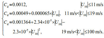 (5)
(5)Furthermore, in Eq.3, θ is the deflection of Ekman flow relative to the wind direction, B is the amplitude coefficient. Assuming constant eddy viscosity, classical Ekman theory indicates that the wind drift spiral and decay with depth, and θ is 45° on the ocean surface. Bressan and Constantin (2019) have proposed a perturbative approach, which provide a formula for the deviation of the deflection angle from the 45° reference value. Constantin et al. (2020) have investigated the deflection angle of wind drift relative to the surface wind stress based on the vertically varying eddy viscosity. In this paper, we did not use such a sophisticated analysis. Instead, to compare directly with ocean surface current at 15-m depth, we use the regression results in Lagerloef et al. (1999), which is calculated based on satellite data and in-situ observations. In the regions between 5°N and 25°N, B and θ can be estimated as
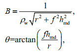 (6)
(6)in which ρw is the water density (ρw=1.025×10³kg/m3), r is the frictional coefficient (r=2.15×10⁻⁴ m/s) and hmd is the mixing depth (hmd=32.5 m). While in the region away from 25°N, both B and θ are taken as constants as B=0.3 m/(s∙Pa), θ=±55° (which means that in the region north of 25°N in the Northern Hemisphere, the classical Ekman current turns 55° to right of the wind). The variations of B and θ with latitudes are shown in Fig. 2, which presents that both B and θ show a jump at the 25°N latitude and this is not consistent with the real world ocean. To solve the drawbacks, weight functions of F10 and F25 are introduced in this paper to improve the Ekman current formulation based on the method of An et al. (2013). The re-constructed Ekman current formulation in different latitude bands are expressed as
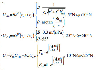 (7)
(7)

|
| Fig.2 The amplitude coefficient B (a) and the turning angle of the classical Ekman current relative to the wind (b) |
The variations of the two weight coefficients are shown in Fig. 3, showing that while the latitude approximates 10°N, F10 (Fig. 3a) approaches 1 and F25 (Fig. 3b)approaches 0, while the latitude approximates 25°N, F10 approaches 0 and F25 approaches 1. The incorporation of the two parameters may probably improve the Ekman current calculation to a certain extent.

|
| Fig.3 Weight coefficients of the Ekman formulation a. F10; b. F25. |
The wave-induced current can be estimated from the following equation (Liu et al., 2007; Wu and Liu, 2008; Hui and Xu, 2016)
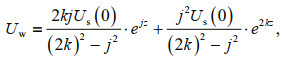 (8)
(8)in which 
 (9)
(9)where Us(0) is the surface Stokes drift velocity, a is the wave amplitude and a=1/2Hs (Hs is the significant wave height), σ is the wave frequency, and k is the wave number. 

 (10)
(10)where T is the mean wave period provided by the ERA-Interim Reanalysis wave data.
2.2.4 Error analysisTo access the quality of wave-modified ocean surface currents, the root mean square error (RMSE) between estimated and in-situ values is calculated as
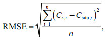 (11)
(11)where Cs, i and Csitu, i are the estimated and in-situ zonal (meridional) ocean surface current at time i respectively, n is the length of time. RMSE values can also be normalized based on the standard deviation of the in-situ observations as
 (12)
(12)where Csitu is the averaged in-situ surface current observations. NRMSE (normalized RSME) was used in this study as a measure of the accuracy of the wavemodified ocean surface currents and lower NRMSE values would indicate higher accuracy.
3 RESULTThe 6-hourly, 0.25°×0.25° gridded ocean surface currents with wave effects in the northwestern Pacific Ocean are estimated based on the methods in Section 2.2, which include geostrophic current from the MADT, classical Ekman current from the CCMP wind speed, and the wave-induced current estimated from the ERA-Interim surface wave datasets. This wave-modified ocean surface currents are validated by comparing with in-situ data from Lagrangian drifters in the study area and KEO observations (32.3°N, 144.6°E) moored at 15-m depth. Before comparison, the gridded wave-modified ocean surface currents are temporal and spatial interpolated to each drifter current vector and KEO observations both for zonal and meridional components. Detailed analysis are shown in Sections 3.1 and 3.2.
3.1 Comparison with Lagrangian drifterIn this section, validations are performed using Lagrangian drifter observations in the northwestern Pacific Ocean from 1 January 1993 to 31 December 2017. To present the spatial distributions of the comparison results, we have binned all the corresponding data into 1°×1° resolution boxes. Figure 4 is the averaged result, which presents that wave-modified ocean surface currents (Fig. 4a) agree well with drifter observations (Fig. 4b) in most of the northwestern Pacific Ocean, especially in deep water regions away from the coast, where ocean surface currents are barely affected by the terrain. Furthermore, the Kuroshio flow path at the depth of 15 m is well characterized, which is quite similar between wavemodified currents and drifter observations. However, there still exist some discrepancies. The wavemodified ocean surface currents underestimate in-situ drifter observations in amplitude, while current directions are almost consistent. Especially in the Luzon Strait, northeast of Taiwan, China, as well as regions along the south coast of the Honshu island and southeast of the Mindanao. There are two possible reasons for this phenomenon. One is that drifter velocity is a combination of a series of current vectors, which includes geostrophic current and ageostrophic flow. Except for the classical Ekman current and the wave-induced current, this ageostrophic flow also contains many other current terms, which cannot be retrieved using these limited datasets mentioned in this article alone. And another reason is that these regions are near the coast and terrain is an important factor affecting the accuracy of ocean surface currents, which needs to be taken into account in the future analysis.

|
| Fig.4 Ocean surface currents averaged from 1993 to 2017 a. wave-modified ocean surface currents; b. Lagrangian drifter currents. Colors represent the magnitude of current velocity, and arrows represent the direction. |
To evaluate the quality of the wave-modified current products, we have estimated correlation and NRMSE in each grid point. To reduce the errors, only effective drifter observations exceeding 30 in each grid point are used. The zonal and meridional correlations between 6-hourly wave-modified ocean surface currents and Lagrangian drifter observations from 1993 to 2017 are shown in Fig. 5a–b respectively. Result shows that in the northwestern Pacific Ocean, the zonal (meridional) correlation exceeding 0.5 occupies about 96.9% (92.3%) of the ocean, and zonal correlations are higher than the meridional component for most of the ocean, especially in the Kuroshio and Kuroshio Extension regions. This is probably caused by the strong geostrophic current, which is the main current component in this area and the method for calculating this velocity is particularly mature. While for the ageostrophic current, there are still some complex unknown elements, which need to be explored in the future studies.

|
| Fig.5 Correlations between wave-modified ocean surface currents and Lagrangian drifter observations from 1993 to 2017 a. zonal component; b. meridional component. |
To assess and compare the errors between estimated ocean surface currents and in-situ observations in each grid point, we have estimated the NRMSE between wave-modified ocean surface currents and Lagrangian drifter observations for the same period (Fig. 6). The lower NRMSE indicates that the estimated wave-modified ocean surface currents fluctuate within a much smaller range of drifter observed values. Result shows that both for the zonal and meridional components, the NRMSE is lower than 0.8, with much higher values in the low-latitude bands and some offshore regions. What's more, the zonal NRMSE is considerably lower than the meridional component for most of the ocean, which means that the zonal error is smaller than the meridional component. Figure 6 also shows that the pattern of NRMSE is very similar with that of the correlation coefficient (Fig. 5), but presents good negative correlation characteristics. This suggests that the larger the correlation, the smaller the error. To better express the corresponding relationship between correlation and NRMSE, we have shown zonal average of the two validation parameters (Fig. 7), which shows that both for the zonal and meridional components, the correlation (NRMSE) is higher (lower) than 0.55 (0.88). In addition, the zonal correlation (NRMSE) is considerably higher (lower) than the meridional component in the study area. Furthermore, the variation of correlation is negatively correlated with that of the NRMSE, and the correlation coefficient is 0.97 (0.99) for the zonal (meridional) component. The two parameters indicate that our wave-modified ocean surface currents agree well with Lagrangian drifter observations. Moreover, the quality of wave-modified zonal component is relatively higher than that of the meridional component.

|
| Fig.6 NRMSE between wave-modified ocean surface currents and Lagrangian drifter observations from 1993 to 2017 a. zonal component; b. meridional component. |

|
| Fig.7 Zonal average of the correlation and NRMSE between wave-modified ocean surface currents and Lagrangian drifter observations |
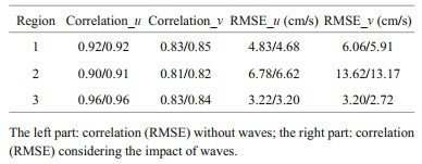
According to the spatial distribution characteristics of the correlation and NRMSE, three representative regions in the study area are selected to do detailed analysis (Fig. 8). To better understand the effects of surface waves, monthly averaged wave-modified ocean surface currents as well as ocean surface currents without waves and Lagrangian drifter observations within each region are calculated (Fig. 9), in which left panels (Fig. 9a1–a3) are the zonal velocity and right panels (Fig. 9b1–b3) are the meridional velocity. Table 1 shows the comparison results of the correlation and RMSE in each region. Our estimates present that considering the impact of waves, the correlation (RMSE) in each region has been increased (decreased), which means that the wave-modified currents are better adapted to in-situ drifter observations than that without waves both for the zonal and meridional components. Nevertheless, the zonal correlation (RMSE) is considerably higher (lower) than that of the meridional component, which means that the coincidence for the zonal component is much better than that of the meridional component. Furthermore, Fig. 9 also shows that the wave-modified ocean surface currents underestimate drifter observations, especially for the meridional component. We estimate that the 1993–2017 averaged velocity in regions 1–3 is 12.77, 17.52, and 14.00 cm/s, respectively, while for the drifter observations, the velocities are 15.02, 21.19, and 14.07 cm/s, respectively. This underestimation is caused by the complex components of drifter observations, which cannot be calculated by finite velocity components in this study. This needs to be revised in the future analysis.

|
| Fig.8 Three selected regions (1, 2, and 3) of the northwestern Pacific Ocean |

|
| Fig.9 Time series of the monthly averaged ocean surface currents without waves (black solid line), wave-modified ocean surface currents (green solid line) and drifter observations (red solid line) of the three representative regions a1–a3. zonal velocity of regions 1, 2, and 3, respectively; b1–b3. meridional velocity of regions 1, 2, and 3, respectively. |
|
Besides, the drifter (ID number 81961) with the maximum life span in the northwestern Pacific Ocean is selected to validate the wave-modified ocean surface currents estimated in this paper, which has 5 076 6-hourly current data points in total and the operating date is from 6 August 2009 to 15 February 2013. The drifter's trajectory is shown in Fig. 10a. In addition, the zonal and meridional scatterplots of ocean surface currents without waves as well as wavemodified ocean surface currents versus drifter observations are shown in Fig. 10b–c & d–e, respectively. This comparison result shows that both the zonal and meridional components of wave-modified ocean surface currents (Fig. 10d–e) coincide better with this Lagrangian drifter observations than that without wave effects. Considering the impact of waves, the correlation (RMSE) has increased (decreased) from 0.85 (17.33 cm/s) to 0.86 (16.52 cm/s) for the zonal component and from 0.83 (16.01 cm/s) to 0.84 (15.65 cm/s) for the meridional component. The much higher correlation and lower NRMSE for the zonal component is consistent with the above analysis. Furthermore, the higher RMSE and NRMSE for this comparison may have two important reasons. One is that some floating areas of this selected drifter are near the coast, and terrain becomes an important factor affecting the accuracy of wave-modified ocean surface currents. The other is that the ocean surface circulation in the Kuroshio and Kuroshio Extension regions are considerably stronger, thus drifter velocities have been underestimated much larger than low current regions.

|
| Fig.10 The comparison between calculated ocean surface currents and the drifter (ID number 81961) with the maximum life span in the northwestern Pacific Ocean a. trajectory of the drifter; b. scatter plot of the zonal comparison without waves; c. scatter plot of the meridional comparison without waves; d. scatter plot of the zonal comparison with wave effects; e. scatter plot of the meridional comparison with wave effects. |
The comparison between wave-modified ocean surface currents and Lagrangian drifter observations indicates that wave-modified ocean surface currents can generally describe the real world ocean circulation objectively and accurately in the northwestern Pacific Ocean, especially in deep water regions for the zonal component. While in the strong current and offshore regions, especially for the meridional component, the deviations are relatively larger, which need further improvements in our further research. Different correction parameters can be set aiming at different velocity intervals to reduce the errors between wavemodified ocean surface currents and in-situ drifter observations. What's more, as the classical Ekman current representing 15-m depth in this study is derived under the hypothesis of infinite water depth, terrain effect in offshore regions should be taken into account in the future analysis as well.
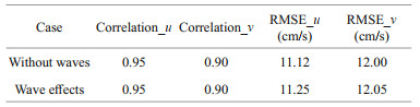
3.2 Comparison with KEO observationsIn this part, the estimated ocean surface currents without waves as well as wave-modified ocean surface currents are compared with KEO observations at 15-m depth from 30 May 2005 to 31 December 2017, with 3 771 available current points in total. Time series of the monthly averaged ocean surface currents is shown in Fig. 11. Result shows that both the zonal (Fig. 11a) and meridional (Fig. 11b) components of the estimated ocean surface currents are consistent with the corresponding KEO observations. However, the direct comparison of the time series both for the zonal and meridional components shown in Fig. 11 cannot clearly illustrate the effects of surface waves. Therefore, we provide the correlation and RMSE between the ocean surface currents without waves as well as wave-modified ocean surface currents versus KEO observations, which are listed in Table 2 in detail. Result shows that the correlation (RMSE) is 0.95 (11.12 cm/s) for the zonal component and 0.90 (12.00 cm/s) for the meridional component between ocean surface currents without waves and KEO observations. While for the wave-modified ocean surface currents, the RMSE is 11.25 cm/s for the zonal comparison and 12.05 cm/s for the meridional comparison. This result manifests that considering the impact of waves, the error between the estimated ocean surface currents and KEO observations becomes larger. This is probably due to the fixed point observations of the KEO, which merely represents the Eulerian current and does not consider the impact of waves.

|
| Fig.11 Comparisons of the estimated ocean surface currents with KEO observations located at 32.3°N, 144.6°E, 15-m depth a. zonal component; b. meridional component. |
|
Histograms of differences between wave-modified ocean surface currents and KEO observations are presented in Fig. 12. Result shows that percentages of the difference approaching zero are the highest both for zonal and meridional components, which is 29.81% and 25.62% respectively. In addition, the difference approaching ±10 cm/s takes the second place, which is 41.02% and 39.70%. The difference between ±40 and ±60 cm/s is 6.05% (7.80%) for the zonal (meridional) component. High rates within a smaller error range (lower than ±20 cm/s) for the zonal (88.01%) and meridional (84.22%) components means that our wave-modified ocean surface currents can better describe the zonal and meridional components of the KEO observations, especially for the zonal component.

|
| Fig.12 Histograms of the difference between wave-modified ocean surface currents and KEO observations a. zonal component; b. meridional component. |
By incorporating the wave-induced CoriolisStokes forcing into the classical Ekman model, wavemodified ocean surface currents in the northwestern Pacific Ocean were calculated based on the CMEMS MADT, CCMP wind speed, and ERA-Interim surface wave datasets from 1 January 1993 to 31 December 2017. Weight functions of F10 and F25 were introduced in the Ekman current formulation as well. The current products were validated by comparing the in-situ data from Lagrangian drifters and KEO observations moored at 32.3°N, 144.6°E, 15-m depth.
Result shows that the modified ocean surface currents are in good agreement with in-situ observations, especially for the zonal component. The comparison with Lagrangian drifter observations indicates that by considering the impact of waves, the estimated ocean surface currents have been improved compared with that without waves. Moreover, the zonal (meridional) correlation exceeding 0.5 occupies about 96.9% (92.3%) of the ocean. Furthermore, the monthly comparison with KEO observations at 15-m depth demonstrates that the wave-modified currents are consistent with KEO observations and the zonal (meridional) correlation and RMSE are 0.95 (0.90) and 11.25 cm/s (12.05 cm/s) respectively. Even so, there still exist some discrepancies. Our wavemodified ocean surface currents underestimate the Lagrangian drifter velocities, especially in the strong current and some offshore regions, but overestimate the KEO observations in some individual months. The reasons are as follows. Drifter velocity represents the Lagrangian motion, which contains a complex set of current components. However, some of these components have not been included in our wavemodified products except for the classical Ekman current, geostrophic current, and the wave-induced current, all of which needs further research in the future studies. Furthermore, this discrepancy between wave-modified currents and drifter observations is mainly situated in offshore regions, where complex topography and shallow waters may have a great impact on the accuracy of ocean surface currents retrieval. The KEO observations are the Eulerian mean currents, which do not include the Stokes drift. Next step, we plan to work out an ocean surface current retrieval method based on the satellite remote sensing data, high precision bathymetric topographic data and in-situ observations, which may provide more reliable ocean surface current products in the future study.
5 DATA AVAILABILITY STATEMENTThe MADT data is provided by CMEMS (http://marine.copernicus.eu/services-portfolio/access-toproducts/?option=com_csw&view=details&product_id=SEALEVEL_GLO_PHY_L4_REP_OBSERVATIONS_008_047) and is downloaded from ftp://my.cmemsdu.eu/Core/SEALEVEL_GLO_PHY_L4_REP_OBSERVATIONS_008_047/dataset-duacs-rep-globalmerged-allsat-phy-l4. The CCMP Version-2.0 vector wind is produced by the Remote Sensing Systems. Data are available at: http://data.remss.com/ccmp/v02.0/. The ERA-Interim surface wave data is downloaded from http://apps.ecmwf.int/datasets/data/interim-full-daily. The in-situ Lagrangian drifter currents are downloaded from https://www.aoml.noaa.gov/phod/gdp/. The in-situ KEO observations are available at https://www.pmel.noaa.gov/ocs/data/disdel/.
An Y Z, Chen Y D, Zhang R, Wang H Z, Chen J. 2013. Ocean surface currents retrieval based on the satellite remote sensing data. Marine Science Bulletin, 15(2): 46-58.
DOI:10.3969/j.issn.1000-9620.2013.02.005 |
Boccaletti G, Ferrari R, Adcroft A, Ferreira D, Marshall J. 2005. The vertical structure of ocean heat transport. Geophysical Research Letters, 32(10): L10603.
DOI:10.1029/2005gl022474 |
Bonjean F, Lagerloef G S F. 2002. Diagnostic model and analysis of the surface currents in the Tropical Pacific Ocean. Journal of Physical Oceanography, 32(10): 2938-2954.
DOI:10.1175/1520-0485(2002)032<2938:DMAAOT>2.0.CO;2 |
Bressan A, Constantin A. 2019. The deflection angle of surface ocean currents from the wind direction. Journal of Geophysical Research: Oceans, 124(11): 7412-7420.
DOI:10.1029/2019JC015454 |
Brickman D, Frank K T. 2000. Modelling the dispersal and mortality of Browns Bank egg and larval haddock (Melanogrammus aeglefinus). Canadian Journal of Fisheries and Aquatic Sciences, 57(12): 2519-2535.
DOI:10.1139/f00-227 |
Constantin A, Dritschel D G, Paldor N. 2020. The deflection angle between a wind-forced surface current and the overlying wind in an ocean with vertically varying eddy viscosity. Physics of Fluids, 32(11): 116604.
DOI:10.1063/5.0030473 |
Dohan K, Maximenko N. 2010. Monitoring Ocean Currents with Satellite Sensors. 2010. Oceanography (Washington D.C.), 23(4): 94-103.
DOI:10.5670/oceanog.2010.08 |
Dohan K. 2017. Ocean surface currents from satellite data. Journal of Geophysical Research: Oceans, 122(4): 2647-2651.
DOI:10.1002/2017JC012961 |
Du Y, Dong X L, Jiang X W, Zhang Y H, Zhu D, Sun Q W, Wang Z Z, Niu X H, Chen W, Zhu C, Jing Z Y, Tang S L, Li Y N, Chen J, Chu X Q, Xu C, Wang T Y, He Y H, Han B, Zhang Y, Wang M Y, Wu W, Xia Y F, Chen K, Qian Y K, Shi P, Zhan H G, Peng S Q. 2021. Ocean surface current multiscale observation mission (OSCOM): simultaneous measurement of ocean surface current, vector wind, and temperature. Progress in Oceanography, 193: 102531.
DOI:10.1016/j.pocean.2021.102531 |
Ekman V W. 1905. On the influence of the earth's rotation on ocean-currents. Arkiv för Matematik, Astronomi och Fysik, 2(11): 1-53.
|
Esselborn S, Eden C. 2001. Sea surface height changes in the North Atlantic Ocean related to the North Atlantic Oscillation. Geophysical Research Letters, 28(18): 3473-3476.
DOI:10.1029/2001GL012863 |
Frankignoul C, Bonjean F, Reverdin G. 1996. Interannual variability of surface currents in the tropical Pacific during 1987-1993. Journal of Geophysical Research: Oceans, 101(C2): 3629-3647.
DOI:10.1029/95JC03439 |
Gao J, Mu L, Bao X W, Song J, Ding Y. 2018. Drift analysis of MH370 debris in the southern Indian Ocean. Frontiers of Earth Science, 12(3): 468-480.
DOI:10.1007/s11707-018-0693-0 |
Hansen D V, Poulain P M. 1996. Quality control and interpolations of WOCE-TOGA drifter data. Journal of Atmospheric and Oceanic Technology, 13(4): 900-909.
DOI:10.1175/1520-0426(1996)013<0900:QCAIOW>2.0.CO;2 |
Hasselmann K. 1970. Wave-driven inertial oscillations. Geophysical Fluid Dynamics, 1(3-4): 463-502.
DOI:10.1080/03091927009365783 |
Henry D. 2019. Stokes drift in equatorial water waves, and wave-current interactions. Deep Sea Research Part II: Topical Studies in Oceanography, 160: 41-47.
DOI:10.1016/j.dsr2.2018.08.003 |
Hui Z L, Xu Y S. 2016. The impact of wave-induced Coriolis-Stokes forcing on satellite-derived ocean surface currents. Journal of Geophysical Research: Oceans, 121(1): 410-426.
DOI:10.1002/2015JC011082 |
Lagerloef G S E, Lukas R, Bonjean F, Gunn J T, Mitchum G T, Bourassa M, Busalacchi A J. 2003. El Niño Tropical Pacific Ocean surface current and temperature evolution in 2002 and outlook for early 2003. Geophysical Research Letters, 30(10): 1514.
DOI:10.1029/2003GL017096 |
Lagerloef G S E, Mitchum G T, Lukas R B, Niiler P P. 1999. Tropical Pacific near-surface currents estimated from altimeter, wind, and drifter data. Journal of Geophysical Research: Oceans, 104(C10): 23313-23326.
DOI:10.1029/1999JC900197 |
Large W G, Pond P. 1981. Open ocean momentum flux measurements in moderate to strong winds. Journal of Physical Oceanography, 11(3): 324-336.
DOI:10.1175/1520-0485(1981)011<0324:OOMFMI>2.0.CO;2 |
Lee T, Hakkinen S, Kelly K, Qiu B, Bonekamp H, Lindstrom E J. 2010. Satellite observations of ocean circulation changes associated with climate variability. Oceanography, 23(4): 70-81.
DOI:10.5670/oceanog.2010.06 |
Lewis D M, Belcher S E. 2004. Time-dependent, coupled, Ekman boundary layer solutions incorporating Stokes drift. Dynamics of Atmospheres and Oceans, 37(4): 313-351.
DOI:10.1016/j.dynatmoce.2003.11.001 |
Liu B, Wu K J, Guan C L. 2007. Global estimates of wind energy input to subinertial motions in the Ekman-Stokes layer. Journal of Oceanography, 63(3): 457-466.
DOI:10.1007/s10872-007-0041-6 |
Lumpkin R, Grodsky S A, Centurioni L, Rio M H, Carton J A, Lee D. 2013. Removing spurious low-frequency variability in drifter velocities. Journal of Atmospheric and Oceanic Technology, 30(2): 353-360.
DOI:10.1175/JTECH-D-12-00139.1 |
Lumpkin R, Johnson G C. 2013. Global ocean surface velocities from drifters: mean, variance, El Niño-Southern Oscillation response, and seasonal cycle. Journal of Geophysical Research: Oceans, 118(6): 2992-3006.
DOI:10.1002/jgrc.20210 |
Lumpkin R, Pazos M. 2007. Measuring surface currents with Surface Velocity Program drifters: the instrument, its data, and some recent results. Lagrangian Analysis and Prediction of Coastal and Ocean Dynamics, 39.
DOI:10.1017/CBO9780511535901.003 |
Matthews J P, Ostrovsky L, Yoshikawa Y, Komori S, Tamura H. 2017. Dynamics and early post-tsunami evolution of floating marine debris near Fukushima Daiichi. Nature Geoscience, 10(8): 598-603.
DOI:10.1038/ngeo2975 |
Morinta I, Sugioka S I, Kojima T. 1997. Real-time forecasting model of oil spill spreading. 1997. International Oil Spill Conference Proceedings, 1997(1): 559-566.
DOI:10.7901/2169-3358-1997-1-559 |
Niiler P P, Paduan J D. 1995. Wind-driven motions in the northeast Pacific as measured by Lagrangian drifters. Journal of Physical Oceanography, 25(11): 2819-2830.
DOI:10.1175/1520-0485(1995)025<2819:WDMITN>2.0.CO;2 |
Pazan S E, Niiler P P. 2001. Recovery of near-surface velocity from undrogued drifters. Journal of Atmospheric and Oceanic Technology, 18(3): 476-489.
DOI:10.1175/1520-0426(2001)018<0476:RONSVF>2.0.CO;2 |
Phillips O M. 1977. The Dynamics of the Upper Ocean. 2nd edn. Cambridge University Press, Cambridge, UK. 336p.
|
Picaut J, Hackert E, Busalacchi A J, Murtugudde R, Lagerloef G S E. 2002. Mechanisms of the 1997-1998 El Niño—La Niña, as inferred from space-based observations. Journal of Geophysical Research: Oceans, 107(C5): 5-1-5-18.
DOI:10.1029/2001JC000850 |
Polton J A, Lewis D M, Belcher S E. 2005. The role of wave-induced Coriolis-Stokes forcing on the wind-driven mixed layer. Journal of Physical Oceanography, 35(4): 444-457.
DOI:10.1175/JPO2701.1 |
Price J F, Sundermeyer M A. 1999. Stratified Ekman layers. Journal of Geophysical Research: Oceans, 104(C9): 20467-20494.
DOI:10.1029/1999JC900164 |
Reiss C S, Panteleev G, Taggart C T, Sheng J, deYoung B. 2000. Observations on larval fish transport and retention on the Scotian Shelf in relation to geostrophic circulation. Fisheries Oceanography, 9(3): 195-213.
DOI:10.1046/j.1365-2419.2000.00139.x |
Reverdin G, Frankignoul C, Kestenare E, McPhaden M J. 1994. Seasonal variability in the surface currents of the equatorial Pacific. Journal of Geophysical Research: Oceans, 99(C10): 20323-20344.
DOI:10.1029/94JC01477 |
Santiago-Mandujano F, Firing E. 1990. Mixed-layer shear generated by wind stress in the central equatorial Pacific. Journal of Physical Oceanography, 20(10): 1576-1582.
DOI:10.1175/1520-0485(1990)020<1576:MLSGBW>2.0.CO;2 |
Sikhakolli R, Sharma R, Basu S, Gohil B S, Sarkar A, Prasad K V S R. 2013a. Evaluation of OSCAR ocean surface current product in the tropical Indian Ocean using in situ data. Journal of Earth System Science, 122(1): 187-199.
DOI:10.1007/s12040-012-0258-7 |
Sikhakolli R, Sharma R, Kumar R, Gohil B S, Sarkar A, Prasad K V S R, Basu S. 2013b. Improved determination of Indian Ocean surface currents using satellite data. Remote Sensing Letters, 4(4): 335-343.
DOI:10.1080/2150704X.2012.730643 |
Smith P C, Lawrence D J, Thompson K R, Sheng J, Verner G, James J St, Bernier N, Feldman L. 1998. Improving the skill of search and rescue forecasts. Canadian Meteorological and Oceanographic Society Bulletin, 26(5): 119-129.
|
Song J B. 2009. The effects of random surface waves on the steady Ekman current solutions. Deep Sea Research Part I: Oceanographic Research Papers, 56(5): 659-671.
DOI:10.1016/j.dsr.2008.12.014 |
Stokes G G. 1847. On the theory of oscillatory waves. Transactions of the Cambridge Philosophical Society, 8: 441-473.
|
Sudre J, Maes C, Garçon V. 2013. On the global estimates of geostrophic and Ekman surface currents. Limnology and Oceanography: Fluids and Environments, 3(1): 1-20.
DOI:10.1215/21573689-2071927 |
Sudre J, Morrow R A. 2008. Global surface currents: a high-resolution product for investigating ocean dynamics. Ocean Dynamics, 58(2): 101.
DOI:10.1007/s10236-008-0134-9 |
Tang C L, Gui Q. 1996. A dynamical model for wind-driven ice motion: application to ice drift on the Labrador Shelf. Journal of Geophysical Research: Oceans, 101(C12): 28343-28364.
DOI:10.1029/96JC02661 |
Trinanes J A, Olascoaga M J, Goni G J, Maximenko N A, Griffin D A, Hafner J. 2016. Analysis of flight MH370 potential debris trajectories using ocean observations and numerical model results. Journal of Operational Oceanography, 9(2): 126-138.
DOI:10.1080/1755876X.2016.1248149 |
van den Bremer T S, Breivik ø. 2018. Stokes drift. Philosophical Transactions of the Royal Society A: Mathematical, Physical and Engineering Sciences, 376(2111): 20170104.
DOI:10.1098/rsta.2017.0104 |
van Sebille E, Aliani S, Law K L, Maximenko N, Alsina J M, Bagaev A, Bergmann M, Chapron B, Chubarenko I, Cózar A, Delandmeter P, Egger M, Fox-Kemper B, Garaba S P, Goddijn-Murphy L, Hardesty B D, Hoffman M J, Isobe A, Jongedijk C E, Kaandorp M L A, Khatmullina L, Koelmans A A, Kukulka T, Laufkötter C, Lebreton L, Lobelle D, Maes C, Martinez-Vicente V, Maqueda M A M, Poulain-Zarcos M, Rodríguez E, Ryan P G, Shanks A L, Shim W J, Suaria G, Thiel M, van den Bremer T S, Wichmann D. 2020. The physical oceanography of the transport of floating marine debris. Environmental Research Letters, 15(2): 023003.
DOI:10.1088/1748-9326/ab6d7d |
Wu K J, Liu B. 2008. Stokes drift-induced and direct wind energy inputs into the Ekman layer within the Antarctic Circumpolar Current. Journal of Geophysical Research: Oceans, 113(C10): C10002.
DOI:10.1029/2007JC004579 |