 2022, Vol. 40
Institute of Oceanology, Chinese Academy of Sciences
Article Information
- LIU Kai, GAO Shan, WANG Fan
- Deviation of the Lagrangian particle tracing method in the evaluation of the Southern Hemisphere annual subduction rate
- Journal of Oceanology and Limnology, 40(3): 891-906
- http://dx.doi.org/10.1007/s00343-021-1097-7
Article History
- Received Mar. 25, 2021
- accepted in principle May. 6, 2021
- accepted for publication Jul. 27, 2021


2 Center for Ocean Mega-Science, Chinese Academy of Sciences, Qingdao 266071, China;
3 University of Chinese Academy of Sciences, Beijing 100049, China;
4 China Laboratory for Ocean Dynamics and Climate, Pilot National Laboratory for Marine Science and Technology (Qingdao), Qingdao 266237, China
An important part of the ventilated thermocline theory (e.g., Iselin, 1939; Stommel, 1979; Luyten et al., 1983; Pedlosky and Young, 1983; Huang, 1990) is the subduction process of upper ocean water. The subduction process refers to the ocean dynamic process in which the water in the mixed layer is detrained into the permanent thermocline along the isopycnal surface under the effect of buoyancy forcing, for example, surface cooling, and flows into the subsurface and deeper layers to participate in thermohaline circulation. Because the abrupt deepening of the mixed layer mainly occurs in late winter, subduction is taken as an intermittent process (Stommel, 1979; Williams et al., 1995), in which subducted water is selected by a "demon", which is known as "Stommel's demon". Cushman-Roisin (1987) further divided the water exchange between the mixed layer and thermocline into three periods: late winter to early spring, early spring to early autumn, and early autumn to late winter. During the period from early spring to early autumn, the water detrained from the mixed layer usually only enters the seasonal thermocline. When the mixed layer becomes deeper, this water is most likely re-entrained back into the mixed layer; therefore, this is not effective subduction. During the period from early autumn to late winter, along with the deepening of the mixed layer, the subsurface water continuously entrains into the mixed layer through the bottom of the mixed layer. This process is called entrainment. According to Stommel's hypothesis, the short period between late winter and early spring is a period of effective subduction when the water in the mixed layer enters the permanent thermocline where is too deep for water to re-entrain into the mixed layer. Since only the effectively subducted water mass will carry the surface seawater characteristics into the subsurface layer and then into the meridional overturning circulation (MOC), it is particularly important to estimate the effective subduction rate precisely.
In general, the mode water originating from the subduction process is considered the source of ocean thermohaline circulation and has a very important contribution to its formation and variation. Therefore, many previous studies have focused on the subduction process of mode waters. For example, in the subtropical gyre, subducted mode waters transport heat and salt from the subtropics to the tropics (McCreary and Lu, 1994). In the subtropical North Atlantic, the large surface density due to the high salinity leads to strong subduction and forms the Subtropical Mode Water (STMW), which thereby participates in the MOC of the North Atlantic (e.g., Häkkinen, 1999; Schott et al., 2003; Zhang et al., 2003) and regulates the global climate. In the subtropical Pacific, the subduction rate of STMWs and Tropical Waters (TWs) and their transport to the equatorial region affect the interannual variability in the El Niño-Southern Oscillation (ENSO) and even the global climate (e.g., Kleeman et al., 1999; Qu et al., 2008; Liu and Wu, 2012; Nie et al., 2016; Tsubouchi et al., 2016; Qu and Gao, 2017). Therefore, the evaluation of the effective subduction rate in different regions is an important approach to study the formation of different mode waters and their variability, and it is also an important way for us to obtain a deeper understanding of the global climate system.
Since the mixed layer in most regions has a significant seasonal cycle, the estimation of the effective subduction rate in most regions is usually calculated in the form of the annual subduction rate (Qiu and Huang, 1995). There are two main methods for calculating the annual subduction rate: one is in the Eulerian frame (henceforth referred to as the "Eulerian method"), and the other is in the Lagrangian frame. The Eulerian method first determines the period of effective subduction within a year and then integrates the local subducted water in the effective period to obtain the annual subduction rate (e.g., De Szoeke, 1980; Cushman-Roisin, 1987; Da Costa et al., 2005; Liu et al., 2016; please see Section 2 for details). This method is accurate in theory; however, it has a great limitation in practical applications: the data used must have a high time resolution. If monthly data are adopted, the accuracy of the effective subduction period is only one month. Most subduction processes occur within 1–2 months during the deep winter (Stommel, 1979; Williams et al., 1995); therefore, the effective period obtained by monthly data is inaccurate. At present, the best observation data that can be used for ocean subduction analysis are gridded Argo data. Since the temporal resolution of Argo data is monthly, Argo data are obviously unsuitable for use in the Eulerian method.
Therefore, the practical method to calculate the annual subduction rate using observation data is the Lagrangian particle tracking method (henceforth referred to as the "Lagrangian method"), as in Qiu and Huang (1995). The Lagrangian method equation for calculating the annual subduction rate Sann is as follows:
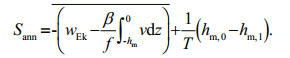 (1)
(1)The first two terms on the right are vertical pumping (VP), which represents the effect of the vertical velocity wmb at the bottom of the mixed layer. The volume of water detrained from the bottom of the mixed layer to the thermocline can then be estimated with wmb; wEk is the Ekman pumping term; and 
However, the Lagrangian method has its own problems. In addition to ignoring the mixing effect (Gao et al., 2011), there are still two noteworthy problems:
1. It assumes that the volume of effective subduction at a given source location is determined by the depth of the particles released at the bottom of the MLD in winter at the source location, which could finally reach a deeper position after one year of tracking, but the actual subduction volume at the source location is not considered.
2. It assumes that Stommel's demon works everywhere (Stommel, 1979). That is, subduction only occurs during a very short period in which the mixed layer rapidly becomes shallow in the deep winter. Therefore, we consider that the water column is almost simultaneously subducted at the source and maintains a straight translational motion at all times (Fig. 1).

|
| Fig.1 Conceptual schematic diagram illustrating the annual subduction rate Eq.1, similar to Fig. 2 in Qiu and Huang (1995) The seasonal change in the mixed layer leads to the emergence of a seasonal pycnocline above the permanent pycnocline. The latitude band is located in a subtropical basin, and the gray water column represents the subducted water. Downward-pointing arrows denote the along-isopycnal geostrophic flows, and the direction to the right represents both equatorward and time for convenience. Ts and Te are the times when effective detrainment starts and ends. Sann is the annual subduction rate, SLI and SVP represent the lateral induction component and the vertical pumping component, respectively. |
Corresponding to the two problems, this method may have two deviations:
1. In fact, the MLD has high spatial variability. If the variation in the MLD at the source location is relatively small, the corresponding possible subduction should also be relatively small. Furthermore, if the winter MLD at the terminal location is very shallow, or the downward Ekman pumping along the particle trajectory is very strong, or the effects of both situations exist at the same time, the subduction volume calculated by the Lagrangian method is likely to be greater than that actually subducted at the source, which will lead to the overestimation of the subduction rate (see Section 3.1 for details).
2. According to a previous study (Williams et al., 1995), Stommel's demon works in the subtropical gyre. However, according to the definition of subduction, effective subduction may not occur only in the deep winter. Imagine some regions where the wind is sufficiently strong, leading to a large downward Ekman pumping; therefore, effective subduction is also likely to occur in periods other than deep winter (see Section 3.2 for details), which is not considered in the Lagrangian method.
To clarify the above issues, we conducted a detailed theoretical analysis and quantitative estimation of these two possible deviations in the Southern Hemisphere. The rest of the paper is organized as follows. A brief description of the data and method of analysis is presented in Section 2. The deviations and their comprehensive deviation are theoretically described and quantitatively estimated in detail in Section 3. Results are summarized in Section 4.
2 MATERIAL AND METHOD 2.1 Argo data and NCEP/NCAR reanalysis wind productArgo data are one of the most important types of ocean observation data at present. Thousands of Argo floats have been deployed since the early 2 000 s to obtain the temperature and salinity (T/S) of the ocean from a typical upper level of 5 m to 2 000 m. By using all qualified Argo profiles, a near real-time, monthly T/S product for the global ocean on a 1°×1° grid has been created by the Asian Pacific Data Research Center (APDRC) of the International Pacific Research Center, University of Hawaii. These data span from January 2005 to the present and have a total of 26 standard vertical levels consistent with those of the World Ocean Atlas (e.g., Levitus, 1983). The climatological monthly Temperature/Salinity data are obtained, from which the geostrophic current of each standard level relative to the non-motion reference level of 2 000 db is calculated. The National Center for Environmental Prediction (NCEP)/National Center for Atmospheric Research (NCAR) reanalysis wind product (Kalnay et al., 1996) is also used for the present study. By using the climatological monthly NCEP wind stress, the Ekman pumping is calculated in this study. The subduction rate is calculated by using these two datasets.
2.2 MLDBased on the climatological Argo T/S data, the climatology of monthly MLD is calculated. The criteria used to define the MLD are diverse in previous studies (e.g., Lindstrom et al., 1987; Lukas and Lindstrom, 1991; Sprintall and Tomczak, 1992; Kara et al., 2000; De Boyer Montégut et al., 2004). According to De Boyer Montégut et al. (2004), the MLD is defined as where the potential density has increased from that of the surface by a density threshold equivalent to a temperature change of 0.5 ℃ at constant salinity. The density threshold can be expressed as
 (2)
(2)in which T0 m, S0 m, and P0 are the local surface temperature, salinity, and pressure, respectively.
2.3 The jet propulsion laboratory (JPL) "off-line" simulated tracer methodThe off-line simulated tracer method of Fukumori et al. (2004) is used to calculate the annual subduction rate in the Southern Hemisphere. In this method, precomputed velocity and mixing tensors are used to integrate the model's advection-diffusion equation. In the context of a general circulation model, the temporal evolution of a passive tracer is determined by the same advection-diffusion equation as that for temperature and salinity, except for differences in possible tracer sources and sinks and in external forcing and boundary conditions:
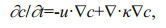 (3)
(3)where c is the tracer concentration, u is the threedimensional velocity vector, and κ is the mixing tensor. If a particular patch of water is uniformly initialized with a passive tracer, the subsequent movement of this tracer will indicate the pathway and destination of the initial patch of water. In particular, the magnitude of the tracer at a given location relative to the value of the initial patch describes the concentration of this initial water mass at the given location. While passive tracers can trace where tracertagged water goes, the adjoint passive tracer that is integrated backward in time can identify where the adjoint tracer-tagged water comes from. Mathematically, a quantity's adjoint is the sensitivity of that quantity to other variables. In particular, the adjoint passive tracer is defined as the sensitivity of a passive tracer at a given location (target) and at a given time (terminal instant) to tracers at other locations at earlier instances. Such sensitivity will be finite if and only if water from such a location makes its way to the target at the terminal instant. Therefore, the value of this sensitivity relative to that of the target describes the fraction of water that circulates from that location to the target location. Please refer to Fukumori et al. (2004) for details.
The annual subduction rate that includes the effect of mixing in addition to advection can be analyzed using this simulated adjoint tracer method. An adjoint tracer is initialized in September (austral winter) with a unit value (in arbitrary tracer units per volume, ATU/m3) for the entire water volume under the surface mixed layer of the Southern Hemisphere (80°S–0° and 0°–360°E). Using the velocity and mixing tensors of the Estimating the Circulation and Climate of the Ocean (ECCO) simulation, the adjoint tracer is integrated backward in time for 1 year until September of the previous year. The annual subduction rate can then be calculated as
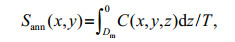 (4)
(4)in which C(x, y, z) is the fraction of tracer-tagged water at position (x, y, z) after the 1-year backward integration, and Dm is the MLD in winter (September) of the previous year. According to this definition, if tracer-tagged water below the winter mixed layer is found re-entering the mixed layer at location A and is traced backward within the mixed layer to location B until the previous winter, it will be regarded as "subducted" at location B. Please refer to Gao et al. (2011) for details.
2.4 The Eulerian methodIn this paper, the deviation in the classical Lagrangian method is corrected by using the Eulerian method. In this method, Sann is defined by the following equation:
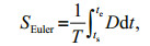 (5)
(5)in which T=1 year and SEuler is the annual subduction rate calculated by Eulerian method, 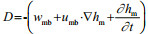
The Eulerian method is theoretically accurate, but the problem is that the determination of its effective detrainment period depends heavily on the time resolution of the data used. Most of the effective subduction occurs during the short period of late winter to early spring, which only lasts for 1–2 months. Therefore, if only monthly data such as Argo data are used, there will be a large deviation in the determination of the effective detrainment period. Therefore, the Eulerian method can only be used to calculate the subduction rate by using model data with high time resolution.
3 RESULTAs analyzed above, two assumptions are used in the classical calculation method of the annual subduction rate:
1. The calculation of the effective subduction is determined by two factors: the new depth of particles after one-year trajectory and the MLD at the location. The amount of the subducted water at the source is not considered.
2. Subduction only occurs in the process of the mixed layer becoming shallower in the deep winter, and possible subduction due to Ekman pumping at other times is not considered.
In the following, we will perform theoretical analysis and quantitative estimation for the possible deviations caused by the above two assumptions.
3.1 Deviation caused by assumption (1)According to Eq.1 for calculating the annual subduction rate by the classical method, a schematic diagram of the corresponding subduction process is given in Fig. 2. It is seen from the figure that the physical process of Eq.1 can be described as follows: the water particle is released at 'O' at the bottom of the mixed layer in the first winter, after moving downstream for one year the particle reaches the new position 'E'. The annual subduction rate is equal to the difference between the depth of 'E' and 'Eh', the 'Eh' is the position of MLD (hm, 1) in the second winter. However, we can see an obvious problem from the figure: the height of the water column representing the subduction rate is actually larger than the real subduction at the source area: Ssource. We can see from the figure that the length of the water column (Oh~O) between the initial position 'O' of the subduction and 'Oh' at the bottom of the summer MLD is the largest possible amount of subduction water at the source in winter of the first year.

|
| Fig.2 Schematic diagram of subduction rate deviation due to insufficient maximum possible subduction water at the source The thin black solid line is sea level, the purple dotted line represents the shallowest MLD in summer, the thick black solid line is the deepest MLD in winter, the black dotted line is realtime MLD, and the thick black arrow represents vertical pumping. Subducted water columns (gray columns) move downwards under the impact of three-dimensional currents U, and the direction to the right represents both equatorward and time. Oh and O are the upper and lower bounds of the initial water column, one year later, the positions of upper and lower bounds become E0 and E. h(min, 0) is the depth of shallowest MLD in summer of first year, h(m, 0) and h(m, 1) are depths of deepest MLD in the first and second winter. Eh is the upper bound of the blue water column Se, which coincides with the deepest MLD h(m, 1) in the second winter. The 42° and 36° are the latitudes. Ssource represent the largest possible amount of subducted water at the source, Sann is the annual subduction rate, and Se is the excess part which is overestimated. |
When the mixed layer suddenly becomes shallower in the source area, there will be a new subducting water column, which will move horizontally due to advection until the winter of the next year and will be affected by Ekman pumping along its path, causing rise or fall in the vertical direction. As shown in Fig. 2, when the dominant direction of Ekman pumping along the path is downward, the subducting water column will sink in the process of downstream movement. However, if the downstream Ekman pumping is large or the downstream winter mixed layer is shallow, the top of the water column (E0) may be compressed under the winter MLD when the water column reaches the position (E~E0) deep in the second winter. Obviously, the water column (Eh~E0) from the top of the water column to the bottom of the mixed layer is not subducted from the source area, so there will be deviation.
Therefore, in which areas will this deviation appear and is this deviation significant? A quantitative analysis of this deviation is performed in the Southern Hemisphere. It can be seen from the analysis that the amount of subducted water masses at the source is determined by three components: first, the mixed layer rapidly becomes shallower in winter, which takes place within 1–2 months after entering the deep winter. Second, the local vertical pumping at the source area also forces the water out of the mixed layer and forms subduction. Third, in these two months, due to the tilt of the mixed layer bottom, the water subducts into the permanent thermocline. Overall, the amount of subduction water masses at the source Ssource can be defined as the local subduction within two months of deep winter, which can be calculated by the Eulerian method:
 (6)
(6)where ts and te are the times when source subduction begins and ends, respectively. As shown in Fig. 3d, the averaged MLD of the South Pacific Ocean and the South Atlantic Ocean represented by the black dotted line begins to shallow after reaching the deepest depth in approximately September, and the period of shallowing usually takes 1 or 2 months. Although the mixed layer in many areas does not reach its shallowest level after the end of this period, the mixed layer generally shallows much more slowly in the next one or two months (Fig. 3d). We believe that after these two months, the subducted water has left the local area due to the current field. Therefore, it is reasonable to set ts and te as the deepest MLD month and two months after that month, respectively; September and November are selected in most areas, but an exception occurs in the sea area south of New Zealand. Due to the influence of unique buoyancy flux characteristics, the spatial variability in MLD is obvious south of New Zealand. The red solid line with triangular symbol denoted 'A' in Fig. 3d identifies a characteristic point (53°S, 168.5°E) in the sea area south of New Zealand, which indicates that the appropriate period of rapid mixed layer shallowing should range from October to December.

|
| Fig.3 The MLD in September in the Southern Hemisphere from Argo gridded climatological data (a); the MLD in March in the Southern Hemisphere from Argo gridded climatological data (b); 101.5°W latitude-depth profiles of MLD in the Southern Hemisphere summer (March) and winter (September) (c); the regional average climatology monthly MLD in the South Pacific (SP, 120°E–60°W, 60°S–10°S) and South Atlantic (SA, 60°W–20°E, 60°S–10°S) Oceans and monthly MLD at A, B, C, and D (d) A (53°S, 168.5°E), B (49°S, 124.5°W), C (19°S, 102.5°W), and D (17°S, 90°E) are four representative points selected for discussion purposes. The positions of these three points also represent three independent areas in the subduction rate pattern, the red vertical line in (a) and (b) denotes the 101.5°W. |
Based on the above discussion, the subduction rate Sann calculated by the classical method cannot be greater than Ssource. If it is greater than the maximum subduction of the source, the excess part is the deviation in the subduction rate, that is,
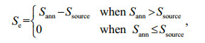 (7)
(7)where Se is the excess part which is overestimated in the calculation of subduction rate.
In the specific analysis, first, according to Eq.1 of the classical method, the annual subduction rate and its components in the Southern Hemisphere are calculated by using the monthly averaged Argo float and NCEP wind field data. Then, according to Eqs.6 and 7, the corresponding deviation is calculated.
Figure 4 shows the spatial distribution of the climatological subduction rate and its vertical pumping and lateral induction components in the Southern Hemisphere. It can be seen from the figure that the subduction area of the South Pacific is mainly concentrated in the subpolar front (60°S–40°S) in the middle latitudes (here the range of middle latitudes is defined as 60°S–30°S) and the subtropical circulation area (25°S–10°S) in the low latitudes (the low latitude range here is 30°S–10°S). Notably, the magnitudes of subduction at different latitudes are different, and subduction at middle latitudes is much larger than that at low latitudes, which is mainly due to the large difference in MLD between low and middle latitudes (Fig. 3). From the component diagrams in Fig. 4b & c, it can be seen that the main component at middle latitudes is the lateral induction term, and vertical pumping plays a relatively small role, while the subduction at low latitudes is different, the vertical pumping term and the lateral induction term have the same magnitude, and subduction is the result of the joint influence of the two components.

|
| Fig.4 Spatial distribution of annual subduction rate (a) and vertical pumping component (b), and lateral induction component (c) in the Southern Hemisphere obtained from monthly averaged Argo float and NCEP wind field data |
Figure 5 shows the spatial distribution of Se and the relative deviation ratio (Se/Sann) in the Southern Hemisphere calculated based on the above considerations. The results indicate that such a situation does exist in the ocean where the maximum subduction of the source in winter is smaller than that calculated by the classical method in some regions. It can also be seen from the contours in Fig. 5a that the significant area is mainly concentrated in the subduction area in the low latitudes, both in the Pacific and Atlantic, from approximately 22°S–10°S, and the absolute deviation in some areas is more than 50 m. The area with high deviation values in the Pacific Ocean is in the same latitude range as that in the Atlantic Ocean; the difference is that the deviation is near the east coast of the Pacific Ocean, while it is near the west coast of the Atlantic Ocean. The high deviation area mainly corresponds to the formation region of STMW characterized by high salinity in the Pacific. In the middle latitudes of the oceans, the deviation is almost zero and can be ignored. This shows that in the middle latitude area, part of the water mass subducted in winter at the source will be entrained back to the downstream mixed layer in the next winter.

|
| Fig.5 Spatial distribution of deviation Se (a) and relative deviation Se/Sann (b) in the Southern Hemisphere Contours show the subduction rates, the values of the interval between the contour lines are 30m, in the latitudes south of 40°S, only the 100-m contours are shown here for comparison with the area where the deviation is located. |
To evaluate the significance of the deviation Se, the estimated value of the relative deviation ratio Se/Sann in the Southern Hemisphere was calculated (Fig. 5b). It can be seen from the figure that the deviation is relatively obvious in the subduction area of the low latitudes. The relative importance in the Pacific and the Atlantic mostly exceeds 30%, and the maximum value can reach 80% (Fig. 5b). Therefore, for low latitudes, the relative deviation in the subduction rate calculated by the classical method cannot be ignored.
Additionally, the seasonal variation in the mixed layer of the Indian Ocean is totally different from that of the Pacific Ocean and the Atlantic Ocean, because it is very obvious that the Indian Ocean is affected by the monsoon, and the MLD may have more than one peak in one year (Liu et al., 2018), as shown by Fig. 3d, two peaks appear in the June (59 m) and December (48.5 m) at the represent point D marked in Fig. 3a in spite of the relative shallow MLD, in the four months after June, the mixed layer became 19 m shallower, and in the two months after December, the mixed layer became shallower by 11.5 m. The two shallowing processes of the mixed layer that occurred within one year will both contribute to the annual subduction rate. Therefore, it is not suitable to use the classical method to calculate the annual subduction rate in the middle and low latitudes of the Indian Ocean. Similarly, the above analysis method is not applicable to the middle and low latitudes of the Indian Ocean. However, a preliminary and conceptual consideration can be made: if the mixed layer has two minimum depths in one year, there will be two effective subduction periods, and the total subduction rate should be the sum of these two processes (Liu et al., 2018, 2020). In each process, the estimation method of the subduction rate is the same as the conventional method, so these two processes should both consider the deviation, and the deviation is more likely to exist in the Indian Ocean than in the Pacific and Atlantic Oceans. However, in this paper, the classical method is used to calculate the Indian Ocean subduction rate, and we do not discuss the deviation results and only give the patterns for reference.
Why does the classical method have no deviation at middle latitudes but obvious deviation at low latitudes? Through the climatological MLD during winter and summer in the Pacific Ocean (Fig. 3c), the reason can be seen. In the middle latitude area, the variation in the MLD is very intense in winter and summer. For example, in the deep winter, the maximum of the MLD at the high subduction point of the middle latitudes (101.5°W–53°S) exceeds 500 m, while in summer, the MLD is only approximately 70 m at the same location. The variation in a year is greater than 400 m, which ensures that the maximum subduction at the source area is very large. At the same time, the vertical pumping in the nearby area is relatively small (Fig. 3b), which ensures that it does not have a great impact on the vertical movement of the subducted water. When the water column reaches the downstream position not far away in the second winter, the deeper mixed layer will inevitably cut off its upper part; that is, there is no deviation Se. However, in the low latitudes, the situation is quite different. First, the difference in MLD between winter and summer is not large. For example, in the deep winter, the deepest mixed layer is 153 m at the maximum position of subduction (19°S–102.5°W) in the low latitudes, while in the summer, it is only 51 m, and the variation range is approximately 100 m (Fig. 3d). In addition, the vertical pumping in this area is much stronger than that in middle-latitude areas (Fig. 4b). As a result, the subducted water column at the source is not sufficient, and the strong vertical pumping along the path will also continuously push the subducted water column downward, and it is likely to completely compress the subducted water column below the winter mixed layer at the end of the second year; that is, deviation Se will be generated.
The question may arise that even if the amount of water at the end exceeds that at the source, this part of the water column is under the mixed layer with certainty, so should it not belong to the effective subduction? Actually, it should be pointed out that due to the existence of the β-spiral, the horizontal current field differs strongly at different depths. Therefore, the water column (Oh~O) that subducted at the time selected by Stommel's demon should be scattered and twisted during the period of moving downstream, instead of always maintaining the original shape of the water column. Additionally, for the water column (Eh~E) at the end point calculated by the Lagrangian method, the water mass may come from the subduction at other positions except for the lowest point, but when we calculate the subduction rate, the effective subducted water mass at the initial position plays a more important role, as that area determines the temperature and salinity characteristics of the subsurface water masses. Therefore, it is not important whether the column obtained by the Lagrangian method comes from the initial position of subduction. The important feature that we care about is to see the difference between the initial subducted water column and the result of the Lagrangian method, that is, the deviation. In other words, the first deviation discussed in our paper is actually a necessary condition; that is, as long as the height of the water column (Eh~E) is greater than that of the equivalent water column (Oh~O) subducted at the source, this deviation must exist in this method.
Furthermore, the Eulerian method is directly used to estimate the water column (Oh~O), that is, the water mass subducted in the selected "Stommel's demon period" is not a cylinder but an equivalent water column height. At the same time, the span of Stommel's demon period is usually only 1–2 months. Due to the limitation of the Eulerian method in resolution, accurate effective subduction is difficult to obtain in monthly results. For example, the effective subduction period in most areas lasts approximately 1.5 months, but 1.5 months cannot be taken as the effective subduction period in the calculation. Therefore, it is impossible to use the exact effective subduction period when using the Eulerian method based on monthly averaged data such as Argo data. Therefore, when calculating the water column (Oh~O) in this study, the effective period is assumed to be two months after the deepest MLD, which is actually a maximum estimation. Therefore, if the subducted column Oh~O obtained by using 2 months as the source Stommel's demon period is less than the result obtained by the Lagrangian method (i.e., the height of the water column Eh~E), then at least the length of Eh~E is overestimated in the subduction calculation.
It should be noted that the MLD is a key factor influencing Sann. The criteria used to define the MLD have been diverse in previous studies (e.g., Lukas and Lindstrom, 1991; Sprintall and Tomczak, 1992; Monterey and Levitus, 1997; Kara et al., 2000; De Boyer Montégut et al., 2004). In some areas where strong subduction exists, the difference of MLD defined by different criteria could be several hundred meters (Piron et al., 2016). Since the lateral induction (LI) is determined by the difference in MLD of the first and second winter, the results of LI calculated by different MLD criteria might be very different. Therefore, it is necessary to further evaluate the sensitivity of the MLD criteria in the calculation of Sann. Due to the space constraint, it will be report in another paper.
In summary, because the classical method does not consider the source subduction, the subduction rate in some of the subduction areas in the low latitudes is overestimated, and there are two reasons for this deviation: (1) there is a large vertical pumping in the subduction area; and (2) there is a small mixed layer change at the source.
3.2 Deviation caused by assumption (2)There is another hypothesis in the classical method: subduction only occurs in the process of the mixed layer becoming shallower in the deep winter and is not considered in other periods; this is also the main assumption of Stommel's demon. In this section, we try to modify this hypothesis based on some considerations to make it more in accordance with the actual physical process in the ocean. First, it should be noted that the vertical pumping considered in the classical method refers to the integral value (the first term of Eq.1 along the trajectory of the particle, which is used to modify the final subduction depth of the particle. However, what we should consider here is the local vertical pumping effect at the source, and the two are different. Because the main component of vertical pumping is Ekman pumping, vertical pumping is a continuous forcing, which is different from MLD variation with its sudden seasonal change. Because of the relatively large fluctuation of the mixed layer in general, the water mass subducted in any season except winter is generally considered to be re-involved in the mixed layer in the winter of the second year, i.e., invalid subduction. However, if the fluctuation in the mixed layer of a specific area is very small and the vertical pumping is very large, there is likely to be effective subduction without re-involvement.
In the following, we will give a detailed description of the mechanism by which vertical pumping contributes a part of the effective subduction rate. As shown in Fig. 6, at a source location 'O' in the Southern Hemisphere, during two months (September, October) entering the deep winter, there will be a rapid shallowing of the mixed layer (Fig. 5b). Therefore, a water mass (gray water column with dotted frame) will subduct below the mixed layer and then move downstream under the influence of advection and vertical pumping and finally reach the point 'E' in the next winter, contributing to effective subduction (solid frame gray water column). This process is the winter subduction process discussed in the previous section. However, in the following time period (November to August of the next year), there is still an opportunity for point 'O' to have effective subduction, which is not considered in the classical method. As shown in the figure, if there is strong vertical pumping locally, point O11 at the bottom of the mixed layer in November may subduct below the mixed layer and move downstream along the horizontal direction. At this time, if there is still a large vertical pumping along the path, the particle will enter a deeper water layer until it reaches a new position E11 in the next winter. If the MLD of this location is shallow in winter, E11 will still be located below the mixed layer, which is an effective subduction. Two conditions are needed for effective subduction: (1) the local pumping and the vertical pumping along the path are relatively strong, and (2) the winter mixed layer at the end point is shallow. By analogy, if the trajectory of water particles at the bottom of the mixed layer is tracked from November to August of the next year, it can be checked whether there is effective subduction in each month. Taking the case in Fig. 6 as an example, at source point 'O', due to the large vertical pumping, water will be detrained out of the mixed layer from November to August of the next year. However, in the next winter, only the water particle from November to February is still under the winter mixed layer, so the subduction water column (thin red strip) in this period is an example of effective subduction, while the subduction water column (thin blue strip) from March to August is an example of invalid subduction.

|
| Fig.6 Schematic diagram of the effect of local vertical pumping for one year on the subduction rate The thin black solid line is sea surface, the black dotted line is the shallowest MLD in summer, the thick black solid line is the deepest MLD in winter, the Ox point represents the water particle at the bottom of the mixed layer in each month at the source, and the Ex point represents the position of each Ox point in the winter of the second year. The subscript x is the corresponding month, U is the three-dimensional currents along the way. The blue line depicts the situation that water subducted at source in February to September in second year cannot pass through the deepest MLD, but the case of red line can form the effective subduction. 42° and 36° are the latitudes. |
Obviously, the analysis of the above subduction process is in accordance with the calculation method of the subduction rate in the Eulerian form, so we can use Eq.5 to estimate the quantity of subducted water in this period. Due to the complexity in each region, the months that can form such a subduction process are not necessarily continuous, as shown in Fig. 6, and there may be discontinuities. Therefore, it is necessary to judge the existence of effective subduction on a monthly basis. Our criterion is that if the water particles in a certain month and the following month are all under the winter mixed layer, then all subducted water masses in that month can be considered effective subduction. In each month, there are two local processes that determine the amount of subduction at the source point O: the local vertical pumping process and changes in the MLD. Therefore, between November and August of the next year, the deviation Svp in the subduction rate caused by vertical pumping at the O point is equal to the sum of subducted water consisting of each effective detrained month. The discretized form of Eq.5 is:
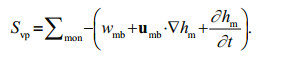 (8)
(8)The subscript "mon" represents the month of effective subduction except the two months that have been considered in Section 3.1. It should also be noted that since the monthly averaged data are used, the effective subduction period obtained by the Eulerian method can only be accurate to one month.
According to Eq.8, Svp in the Southern Hemisphere is also estimated using Argo data and NCEP wind field data, and the results are shown in Fig. 7.

|
| Fig.7 Spatial distribution of deviation Svp in the subduction rate caused by vertical pumping in the Southern Hemisphere (a), with only values greater than 10 shown in color, and relative deviation importance Svp/Sann in the Southern Hemisphere (b) The contour is the subduction rate, the values of the interval between the contour lines are 30 m, in the latitudes south of 40°S, only the 100-m contours are shown here for comparison with the area where the deviation is located. |
Svp is mainly distributed in the low latitudes between 20°S and 10°S, which is very similar to the area of Se in the previous section. The deviation in the east-central Pacific is the most obvious, there is a high value in the latitude band 110°W–130°W, the maximum deviation can exceed 40 m, and the maximum relative importance ratio can reach 70%. However, noticing that the locations of contours represent subduction, the main deviation is not in the typical subduction area, which indicates that the domain of the actual subduction rate is wider if we only consider this deviation. The situation in the Atlantic Ocean is similar, with the large subduction rate area located southwest of the high deviation area. The Svp of the Indian Ocean is smaller but more widespread, and the subduction area calculated by the old method is also widespread in the Indian Ocean (Liu et al., 2018), so it is very likely to have a larger subduction rate if applying the double peak maximum MLD method. Therefore, the deviation in the case of the Indian Ocean is worthy of further investigation. Moreover, Svp is also distributed in some areas in the middle latitudes of the Southern Ocean, especially around the sea south of New Zealand (Fig. 7a). However, it is noteworthy in Fig. 7b that the area with a high deviation ratio is not as wide as the deviation pattern, which is largely due to the high subduction rate in the high deviation area, so the influence of this deviation is not prominent. The main reason for the existence of high Svp in the low latitudes of the Southern Ocean is that the vertical pumping in the low latitudes is strong (Fig. 4b), while the mixed layer is shallow and the fluctuation in MLD is small (Fig. 3d). Under such conditions, vertical pumping will lead to a continuous subduction process in periods other than winter. The magnitude of subduction deviation is particularly large in some low-latitude areas, where it cannot be ignored.
3.3 Comprehensive deviation and correction methodTwo possible deviations in the calculation of the subduction rate by the classical method are analyzed and evaluated. As mentioned above, the conditions for the two deviations are very similar, so they are both located in the low latitudes and have similar influence areas. Therefore, if the two deviations are considered together, some of them compensate for each other, but the total deviation is still significant. We can see from Fig. 8 that the absolute deviation is mainly positive in the main subduction area, which indicates that the overestimation in the classical method of calculating the subduction rate is dominant, and the relative deviation ratio can reach 50% (Fig. 8). In the Pacific Ocean, the deviation is mainly distributed in the eastern Pacific Ocean 160°W–90°W, 20°S–10°S, which corresponds to the subduction area of Eastern Subtropical Mode Water (ESTMW) in the eastern South Pacific. Previous studies have shown that the subduction of ESTMW and its transport to the equator will have an important modulation effect on the climate of the tropical region (Liu and Wu, 2012; Nie et al., 2016; Qu and Gao, 2017), so the deviation in the calculation of the annual subduction rate in this region using the classical method will affect our understanding of this process (Liu and Wu, 2012). In the low latitudes of the Atlantic Ocean, the overestimation of the subduction rate is also obvious, and high values of (Se–Svp)/Sann appear in the area close to the equator. This result reminds us that when using the classical method to calculate the subduction rate, the subduction area in the low latitudes may be inaccurate.

|
| Fig.8 Comprehensive deviation (Se–Svp) (a) and its relative deviation importance (Se–Svp)/Sann in the Southern Hemisphere (b) The contour is the subduction rate, the values of the interval between the contour lines are 30 m, in the latitudes south of 40°S only the 100-m contours are shown here for comparison with the area where the deviation is located. |
To further test the above viewpoint, we use the ECCO model data from the Jet Propulsion Laboratory (JPL) to calculate the subduction rates in the South Pacific Ocean and the South Atlantic Ocean through the classical method and the simulated passive tracer method and compare the two results (Fig. 9). Because the classical method does not consider the role of mixing within the theoretical framework, here, we only show the no-mixing result of the latter method for comparison; more details can be found in Gao et al. (2011). The results clearly show that the two patterns (Fig. 9a & b) are very similar, indicating that the calculation of the subduction rate using the classical method is simple and accurate. However, in the low latitudes of the South Pacific and South Atlantic, the subduction rate obtained by the classical method is obviously larger than that obtained by the simulated passive tracer method, which is consistent with the above deviation analysis (Fig. 9c). Since the subduction rate obtained by the simulated passive tracer method can be regarded as an accurate result, the analysis results of the above two deviations in this paper can explain the difference very well.

|
| Fig.9 Spatial distribution of subduction rates in the South Pacific and South Atlantic calculated using the classical method (a) and ECCO model simulated passive tracer method (no-mixing) (b) and the difference between a and b (c) |
In summary, according to the above analysis and estimation, we can use the Eulerian method to make a preliminary correction for the classical method. The steps are summarized as follows:
1. Use Eq.1 of the classical method to calculate the annual subduction rate Sann.
2. Calculate the local maximum detrained water volume in two months entering the deep winter by using the Eulerian method Eq.6.
3. Use Eq.8 of the Eulerian method to calculate the effective subduction Svp in the following months.
4. Use the two results obtained in steps 2 and 3 to modify the annual subduction rate of the classical method Sann:
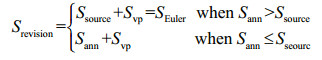 (9)
(9)Please note that the Lagrangian method is not used in Stommel's demon period in the first case, so in areas where both deviations exist, the revised Equation is equivalent to the Eulerian calculation method of the subduction rate: SEuler.
4 DISCUSSIONAs a process of ventilation, subduction relates the properties of the atmosphere with the subsurface water properties of the ocean, which has a considerable impact on the formation and transport of mode water in many regions. Among the world oceans, the Antarctic Circumpolar Current (ACC) plays an important role as a conduit for the interbasin exchange of water masses (Weijer et al., 2012). Through the concept of the Southern Hemisphere super gyre (SHSG), the water properties of the whole Southern Ocean also link together. Then, by the MOC of each ocean, especially the MOC of the Atlantic Ocean, the water masses are globally redistributed. The major water masses involved in these processes, such as Subantarctic Mode Water (SAMW), Antarctic Intermediate Water (AAIW), and Antarctic Bottom Water (AABW), are of great importance to climate change. For example, Gao et al. (2018) pointed out that the heat content related to the global warming hiatus is stored in SAMW and AAIW. Most previous studies focused on the inherent properties of water masses, such as the thickness, depth, and heat content. By calculating the subduction rate, there will be a new way to study the relationship between water masses and climate change from another perspective. Downes et al. (2010) pointed out that the volume of subducted SAMW and AAIW decreases due to the buoyancy gain and shoaling of the winter mixed layer. Qu et al. (2020) studied the variability in SAMW using the subduction rate during the Argo period and found that there is a strong correlation between the quasibiennial variability in SAMW and the Southern Annular Mode (SAM). Therefore, the accurate calculation of the subduction rate has become a precondition to investigate climate change from the perspective of ventilation. Through our research, the special circumstances that may cause deviations are taken into account to ensure effectiveness when using the classical method to calculate the subduction rate of these typical water masses. Apart from the AAIW and SAMW, the subtropical water masses mainly refer to STMW. In the South Pacific, the STMW is more specifically known as ESTMW or South Pacific Eastern Subtropical Mode Water (SPESTMW). SPESTMW spreads northwestward from the ventilation region within the subtropical gyre, eventually joining the South Equatorial Current (Wong and Johnson, 2003; Liu and Wu, 2012). SPESTMW is located at 12S°–24°S and coincides with one of the deviation maxima in the South Pacific, so ESTMW is probably overestimated. Due to the limitations of data and the amount of calculation, the situation in the Northern Hemisphere is not taken into account in this research. However, due to the symmetry of the wind field in the Northern and Southern Hemispheres, it can be predicted that vertical pumping still plays a major role in the formation of STMW in the Northern Hemisphere, and the conditions for the two kinds of deviations will also be satisfied in the tropical and subtropical regions of the Northern Hemisphere, so there should be a similar conclusion. In the area where these deviations exist, Cerovečki and Giglio (2016) and Cerovečki et al. (2019) analyzed the T/S using Argo profiles for 2005 to 2012 and related the decrease in volume of STMW to the change in pycnocline in the formation region, which is closely associated with the subduction process. However, the existence of STMW also has a substantial impact on the pycnocline, and the presence of thick STMW will shoal the upper pycnocline and cause subtropical front (STF) variations on decadal timescales in the North Pacific (Kobashi et al., 2021). As a result, because the main formation regions of SAMW and AAIW are at middle latitudes in the Southern Hemisphere, it is accurate to use the classical tracing method to calculate the subduction rate related to these water masses, but the possible deviations should be accounted for when considering subtropical water masses.
As stated above, the Lagrangian method is dealt with directly when we consider the deviation, but the velocity β-spiral is an unavoidable problem. To solve the problem, there is an effective method, that is, to use high temporal resolution data and the Eulerian method. The Eulerian method is accurate in theory and adopted by many previous studies (e.g., De Szoeke, 1980; Cushman-Roisin, 1987; Liu et al., 2016), but it has a large limitation; that is, it requires a very high temporal resolution of data. For most of the subduction areas, the fluctuation of the mixed layer in the selected Stommel's demon period can reach hundreds of meters. Therefore, the deviation caused by the selection of the effective subduction period determined by the monthly averaged data will be very large, so this scheme is not feasible in practice. One possible approach is to use linear interpolation and directly interpolate the monthly averaged data into quasi-daily averaged data. Considering the Lagrangian tracing process in daily steps, the computational cost would be very high, and the implementation of this method needs to be further simplified in follow-up research. In this paper, the Eulerian method is used in the discussion of the second deviation, that is, to judge whether the subduction in the non-Stommel's demon months is effective. The reason we can use the Argo data with low resolution here is that the fluctuation in MLD is no longer intense in these periods, and the amount of subduction in each month is no longer large, so the absolute deviation in judging the effective period is small. At the same time, as a conservative estimate, only the month of fully effective subduction is considered, so the second deviation is the minimum estimation. In particular, it should be pointed out that the correction Equation of comprehensive deviation (Eq.9) is exactly equivalent to the result of using the complete Eulerian method if the location has both the first deviation and the second deviation. Because at this point, the effective subduction time is longer than the selected Stommel's demon period, so the deviation caused by the time resolution is relatively small.
Further analysis shows that the conditions for the two deviations are similar: strong vertical pumping in the source area and along the path of subduction, as well as MLD with little change. Therefore, the distribution areas of the two deviations are similar but not coincident. Due to the effect of vertical pumping, for the first deviation, vertical pumping along the path is the main influencing factor, which forces the water mass subducted at the source to sink to a very deep depth, thus exceeding the amount of water that the source can produce in winter. For the second deviation, both the vertical pumping along the path and local vertical pumping are very important. The former increases the effective subduction time window, while the latter determines the amount of subducted water that can contribute to the effective subduction window. The small change in the mixed layer also reduces the effect of the lateral induction term and makes the effect of the vertical pumping term more significant.
5 CONCLUSIONUsing low-resolution monthly averaged observation data, at least two possible deviations are discussed in the classical method: the first is that when the mixed layer becomes deeper during the period of the first deep winter, less water may be subducted at the source, which leads to the overestimation of the subduction rate; the other is that the subduction rate may be underestimated without considering subduction during months other than deep winter months at the source. The results of quantitative analysis using Argo and NCEP data show that the two kinds of deviations exist significantly in the low- and middle-latitude subduction areas, their distribution patterns are similar, and they can partially offset each other, but the comprehensive deviation is still significant and cannot be ignored. At middle latitudes, there are almost no such two deviations. The evaluation of these two deviations has distinct physical meanings, and the application of the revised subduction rate in the global ocean will be a meaningful topic for future study.
6 DATA AVAILABILITY STATEMENTThe datasets generated and analyzed during the current study are available from the corresponding author on reasonable request.
7 ACKNOWLEDGMENTThe authors thank all the reviewers for their comments to improve the original manuscript.
Cerovečki I, Giglio D. 2016. North Pacific subtropical mode water volume decrease in 2006-09 estimated from Argo observations: influence of surface formation and basin-scale oceanic variability. Journal of Climate, 29(6): 2177-2199.
DOI:10.1175/JCLI-D-15-0179.1 |
Cerovečki I, Hendershott M C, Yulaeva E. 2019. Strong North Pacific subtropical mode water volume and density decrease in year 1999. Journal of Geophysical Research: Oceans, 124(9): 6617-6631.
DOI:10.1029/2019JC014956 |
Cushman-Roisin B. 1987. Dynamics of the oceanic surface mixed layer. In: Muller P, Henderson D eds. Proceedings of the 'Aha Huliko'a, Hawaiian Winter Workshop. Hawaii Institute of Geophysics, Hawaii. p. 181-196.
|
Da Costa M V, Mercier H, Treguier A M. 2005. Effects of the mixed layer time variability on kinematic subduction rate diagnostics. Journal of Physical Oceanography, 35(4): 427-443.
DOI:10.1175/JPO2693.1 |
De Boyer Montégut C, Madec G, Fischer A S, Lazar A, Iudicone D. 2004. Mixed layer depth over the global ocean: an examination of profile data and a profile-based climatology. Journal of Geophysical Research: Oceans, 109(C2): C12003.
|
De Szoeke R A. 1980. On the effects of horizontal variability of wind stress on the dynamics of the ocean mixed layer. Journal of Physical Oceanography, 10(9): 1439-1454.
DOI:10.1175/1520-0485(1980)010<1439:OTEOHV>2.0.CO;2 |
Downes S M, Bindoff N L, Rintoul S R. 2010. Changes in the subduction of southern ocean water masses at the end of the twenty-first century in eight IPCC models. Journal of Climate, 23(24): 6526-6541.
DOI:10.1175/2010JCLI3620.1 |
Fukumori I, Lee T, Cheng B, Menemenlis D. 2004. The origin, pathway, and destination of Niño-3 water estimated by a simulated passive tracer and its adjoint. Journal of Physical Oceanography, 34(3): 582-604.
DOI:10.1175/2515.1 |
Gao L B, Rintoul S R, Yu W D. 2018. Recent wind-driven change in Subantarctic Mode Water and its impact on ocean heat storage. Nature Climate Change, 8(1): 58-63.
DOI:10.1038/s41558-017-0022-8 |
Gao S, Qu T D, Fukumori I. 2011. Effects of mixing on the subduction of South Pacific waters identified by a simulated passive tracer and its adjoint. Dynamics of Atmospheres and Oceans, 51(1-2): 45-54.
DOI:10.1016/j.dynatmoce.2010.10.002 |
Häkkinen S. 1999. Variability of the simulated meridional heat transport in the North Atlantic for the period 1951–1993. Journal of Geophysical Research: Oceans, 104(C5): 10991-11007.
DOI:10.1029/1999JC900034 |
Huang R X. 1990. On the three-dimensional structure of the wind-driven circulation in the North Atlantic. Dynamics of Atmospheres and Oceans, 15(1-2): 117-159.
DOI:10.1016/0377-0265(90)90006-H |
Iselin C O D. 1939. The influence of vertical and lateral turbulence on the characteristics of the waters at mid-depths. Eos, Transactions American Geophysical Union, 20(3): 414-417.
DOI:10.1029/TR020i003p00414 |
Kalnay E, Kanamitsu M, Kistler R, Collins W, Deaven D, Gandin L, Iredell M, Saha S, White G, Woollen J, Zhu Y, Chelliah M, Ebisuzaki W, Higgins W, Janowiak J, Mo K C, Ropelewski C, Wang J, Leetmaa A, Reynolds R, Jenne R, Joseph D. 1996. The NCEP/NCAR 40-year reanalysis project. Bulletin of the American Meteorological Society, 77(3): 437-472.
DOI:10.1175/1520-0477(1996)077<0437:TNYRP>2.0.CO;2 |
Kara A B, Rochford P A, Hurlburt H E. 2000. An optimal definition for ocean mixed layer depth. Journal of Geophysical Research: Oceans, 105(C7): 16803-16821.
DOI:10.1029/2000JC900072 |
Karstensen J, Quadfasel D. 2002. Formation of southern hemisphere thermocline waters: water mass conversion and subduction. Journal of Physical Oceanography, 32(11): 3020-3038.
DOI:10.1175/1520-0485(2002)032<3020:FOSHTW>2.0.CO;2 |
Kleeman R, McCreary Jr J P, Klinger B A. 1999. A mechanism for generating ENSO decadal variability. Geophysical Research Letters, 26(12): 1743-1746.
DOI:10.1029/1999GL900352 |
Kobashi F, Nakano T, Iwasaka N, Ogata T. 2021. Decadal-scale variability of the North Pacific subtropical mode water and its influence on the pycnocline observed along 137°E. Journal of Oceanography, 77(3): 487-503.
DOI:10.1007/s10872-020-00579-x |
Levitus S. 1983. Climatological Atlas of the World Ocean. US Government Printing Office, Washington.
|
Lindstrom E, Lukas R, Fine R, Firing E, Godfrey S, Meyers G, Tsuchiya M. 1987. The Western Equatorial Pacific Ocean circulation study. Nature, 330(6148): 533-537.
DOI:10.1038/330533a0 |
Liu C Y, Wu L X. 2012. An intensification trend of South Pacific mode water subduction rates over the 20th century. Journal of Geophysical Research: Oceans, 117(C7): C07009.
|
Liu L L, Huang R X, Wang F. 2016. Subduction/obduction rate in the North Pacific diagnosed by an eddy-resolving model. Chinese Journal of Oceanology and Limnology, 34(4): 835-846.
DOI:10.1007/s00343-016-5036-y |
Liu L L, Huang R X, Wang F. 2018. Ventilation of a monsoon-dominated ocean: subduction and obduction in the North Indian Ocean. Journal of Geophysical Research: Oceans, 123(7): 4449-4463.
DOI:10.1029/2017JC013719 |
Liu L L, Huang R X, Wang F. 2020. Ventilation in the South China Sea: subduction versus obduction. Deep Sea Research Part I: Oceanographic Research Papers, 158: 103227.
DOI:10.1016/j.dsr.2020.103227 |
Liu L L, Huang R X. 2012. The global subduction/obduction rates: their interannual and decadal variability. Journal of Climate, 25(4): 1096-1115.
DOI:10.1175/2011JCLI4228.1 |
Lukas R, Lindstrom E. 1991. The mixed layer of the western equatorial Pacific Ocean. Journal of Geophysical Research: Oceans, 96(S01): 3343-3357.
DOI:10.1029/90JC01951 |
Luyten J R, Pedlosky J, Stommel H. 1983. The ventilated thermocline. Journal of Physical Oceanography, 13(2): 292-309.
DOI:10.1175/1520-0485(1983)013<0292:TVT>2.0.CO;2 |
McCreary Jr J P, Lu P. 1994. Interaction between the subtropical and equatorial ocean circulations: the subtropical cell. Journal of Physical Oceanography, 24(2): 466-497.
DOI:10.1175/1520-0485(1994)024<0466:IBTSAE>2.0.CO;2 |
Mill G N, De Moraes Paiva A. 2013. Subduction of South Atlantic subtropical mode waters. Brazilian Journal of Geophysics, 31(3): 495-505.
DOI:10.22564/rbgf.v31i3.323 |
Monterey G, Levitus S. 1997. Seasonal Variability of Mixed Layer Depth for the World Ocean. US Government Printing Office, Washington, DC.
|
Nie X W, Gao S, Wang F, Qu T D. 2016. Subduction of North Pacific Tropical Water and its equatorward pathways as shown by a simulated passive tracer. Journal of Geophysical Research: Oceans, 121(12): 8770-8786.
DOI:10.1002/2016JC012305 |
Pedlosky J, Young W R. 1983. Ventilation, potential-vorticity homogenization and the structure of the ocean circulation. Journal of Physical Oceanography, 13(11): 2020-2037.
DOI:10.1175/1520-0485(1983)013<2020:VPVHAT>2.0.CO;2 |
Piron A, Thierry V, Mercier H, Caniaux G. 2016. Argo float observations of basin-scale deep convection in the Irminger Sea during winter 2011-2012. Deep Sea Research Part I: Oceanographic Research Papers, 109: 76-90.
DOI:10.1016/j.dsr.2015.12.012 |
Qiu B, Huang R X. 1995. Ventilation of the North Atlantic and North Pacific: subduction versus obduction. Journal of Physical Oceanography, 25(10): 2374-2390.
DOI:10.1175/1520-0485(1995)025<2374:VOTNAA>2.0.CO;2 |
Qu T D, Gao S, Fine R A. 2020. Variability of the sub-Antarctic mode water subduction rate during the Argo period. Geophysical Research Letters, 47(13): e2020GL088248.
|
Qu T D, Gao S, Fukumori I, Fine R A, Lindstrom E J. 2008. Subduction of South Pacific waters. Geophysical Research Letters, 35(2): L02610.
|
Qu T D, Gao S. 2017. Resurfacing of South Pacific tropical water in the Equatorial Pacific and its variability associated with ENSO. Journal of Physical Oceanography, 47(5): 1095-1106.
DOI:10.1175/JPO-D-16-0078.1 |
Schott F A, Dengler M, Brandt P, Affler K, Fischer J, Bourlès B, Gouriou Y, Molinari R L, Rhein M. 2003. The zonal currents and transports at 35°W in the tropical Atlantic. Geophysical Research Letters, 30(7): 1349.
|
Sprintall J, Tomczak M. 1992. Evidence of the barrier layer in the surface layer of the tropics. Journal of Geophysical Research: Oceans, 97(C5): 7305-7316.
DOI:10.1029/92JC00407 |
Stommel H. 1979. Determination of water mass properties of water pumped down from the Ekman layer to the geostrophic flow below. Proceedings of the National Academy of Sciences of the United States of America, 76(7): 3051-3055.
DOI:10.1073/pnas.76.7.3051 |
Tsubouchi T, Suga T, Hanawa K. 2016. Comparison study of subtropical mode waters in the world ocean. Frontiers in Marine Science, 3: 270.
|
Weijer W, Sloyan B M, Maltrud M E, Jeffery N, Hecht M W, Hartin C A, Van Sebille E, Wainer I, Landrum L. 2012. The Southern Ocean and its climate in CCSM4. Journal of Climate, 25(5): 2652-2675.
|
Williams R G, Marshall J C, Spall M A. 1995. Does Stommel's mixed layer "Demon" work?. Journal of Physical Oceanography, 25(15): 3089-3102.
|
Wong A P S, Johnson G C. 2003. South Pacific eastern subtropical mode water. Journal of Physical Oceanography, 33(7): 1493-1509.
DOI:10.1175/1520-0485(2003)033<1493:SPESMW>2.0.CO;2 |
Zhang D X, McPhaden M J, Johns W E. 2003. Observational evidence for flow between the subtropical and tropical Atlantic: The Atlantic subtropical cells. Journal of Physical Oceanography, 33(8): 1783-1797.
DOI:10.1175/1520-0485(2003)033<1783:OEFFBT>2.0.CO;2 |