 2022, Vol. 40
Institute of Oceanology, Chinese Academy of Sciences
Article Information
- WANG Sijia, SUN Qun, LI Siyu, SHEN Jiawei, LIU Qian, ZHAO Liang
- Interannual variability of dimethylsulfide in the Yellow Sea
- Journal of Oceanology and Limnology, 40(2): 551-562
- http://dx.doi.org/10.1007/s00343-020-0480-0
Article History
- Received Dec. 24, 2020
- accepted in principle Mar. 17, 2021
- accepted for publication Apr. 30, 2021


2 School of Marine Science and Technology, Tianjin University, Tianjin 300072, China
The most important, abundant, and widespread volatile biogenic sulfur compound in surface seawater is dimethylsulfide (DMS) (Lovelock et al., 1972; Andreae and Barnard, 1984; Andreae et al., 1985). DMS in surface seawater is the source of more than 50% of all natural sulfur emitted into the global atmosphere (Andreae, 1986), and represents a large portion of marine organic volatile emissions (Andreae, 1990). DMS emitted into the atmosphere is rapidly oxidized by OH, NO3, and halogen-oxidized radicals including BrO, IO, and ClO, forming various sulfur-containing products; these sulfur-containing particles are an important source of cloud condensation nuclei (CCN) (Charlson et al., 1987). CCN indirectly affect the Earth's radiative balance by altering the radiative properties of clouds (Nguyen et al., 1992; Andreae and Rosenfeld, 2008), strongly influencing global climate change. Indeed, it has been shown that decreases in sulfur flux as a result of ocean acidification and climate change further exacerbate global warming (Six et al., 2013). Therefore, to better understand climate change, it is important to explore interannual variations in DMS concentration.
Many studies since the 1990s have attempted to hindcast DMS levels in surface seawater based on in-situ observations or using various models in order to analyze interannual variations in DMS concentrations. For example, Song et al. (2019) used an empirical DMS algorithm, and reported that global surface seawater DMS concentrations were stable between 2000 and 2007, but DMS concentrations decreased between 2008 and 2015. In addition, based on the global warming scenarios from 1860 to 2100 outlined by Houghton (2001), Kloster et al. (2007) suggested that global annual mean DMS sea surface concentration and DMS flux will decrease 10% between 1861–1890 and 2061–2090. These studies indicate that the interannual variability in global surface seawater DMS concentration is decreasing.
The DMS emissions from continental shelves form a non-negligible proportion of total global DMS emissions (Gypens and Borges, 2014; Jian et al., 2018; Xu et al., 2019). Although all oceanic continental shelves together represent only 7.5% of total ocean area, the DMS emissions from shelf waters represent about 15.7% of global oceanic DMS emissions (Sciare et al., 2002). River-influenced DMS emissions, which are considered the major factor influencing DMS emission levels in coastal waters, account for about 10% of all DMS emissions from shelf waters (Sciare et al., 2002). In particular, although the European shelves represent only 0.9% of global ocean area, these shelf waters are associated with 2.3% of global oceanic DMS emissions (Uher, 2006). Due to the effects of anthropogenic activities, shelf sea regions are areas of high primary production, with concomitantly high surface seawater DMS concentrations (Yang et al., 2000). The Yellow Sea (YS), which is located at the edge of the northwest Pacific Ocean, is an important shelf sea in China. Yearly variations in DMS concentration in the YS have been extensively investigated. For example, surface seawater DMS concentration in the YS was greater in 2013 than in 2006 (Yang et al., 2011b, 2014); spring DMS concentration in 2006 was also greater than that in 1994 (Yang et al., 2012). Indeed, DMS concentration in the western YS was shown to have increased 2.0–2.8 fold between 2005 and 2012 (Li et al., 2016).
It is difficult to determine the continuous interannual variations in surface seawater DMS concentrations in the YS based on differences in DMS between specific years. Thus, to better clarify ecological and environmental changes in the China Sea, it is important to analyze the characteristics and interannual variations of surface seawater DMS with continuous data. Previously, surface seawater DMS concentrations in the East China Sea (ECS) have been calculated using statistical algorithms (Qu et al., 2020a) and a biogeochemical model (Qu et al., 2020b). To perform a similar long-term continuous surface seawater DMS hindcast in the YS, this study aimed to utilize a generalized additive mixed model (GAMM), in conjunction with satellite sea surface temperature (SST) and local modified chlorophyll-a (LMC) data, to estimate DMS. The interannual variations and trends in DMS, and the factors influencing these trends, are discussed in Section 3.
2 DATA AND METHODOLOGYThe surface seawater DMS concentrations in the YS from 1998 to 2019 were hindcasted using a 22-year GAMM based on satellite SSTs and locally modified Chl-a data. Because DMS could not be estimated with a simple linear model, a GAMM was established with historical in situ data and then used to model the temporal and spatial structures of DMS. The study area covered the entire YS (119°E–127°E, 23°N–40°N), as shown in Fig. 1.

|
| Fig.1 Study region The dashed lines represent boundaries between the Bohai Sea, the YS, and the ECS. |
The 1/4° daily optimum interpolation sea surface temperature (OISST, version 2.1) dataset, produced by the Advanced Very High Resolution Radiometer (AVHRR) from the NOAA National Climatic Data Center (NCDC, http://www.ncdc.noaa.gov/oisst), was processed to obtain the monthly mean SST data. In-situ SST observation data (1998-2001) from two Marine Environment Monitoring Stations, Xiaochangshan station (122.45°E, 39.14°N) and Chengshantou station (122.70°E, 37.23°N), were compared with the SST in AVHRR. The correlation coefficient between the AVHRR SST and in-situ observation data was 0.97.
Standard mapped satellite images from the Ocean Colour Climate Change Initiative dataset (OC-CCI, Version 4.2), produced by the European Space Agency (ESA, http://www.esa-oceancolour-cci.org), were used to derive surface Chl-a concentrations in the YS. The daily LMC in the YS was calculated by establishing a modified model based on OC-CCI and in-situ chlorophyll data; in this modified model, the influence of turbidity was removed (Hao et al., 2019). The correlation coefficient between the LMC and in situ observation data was 0.76.
2.2 GAMM of DMSTo investigate the long-term trends in surface seawater DMS concentration, a GAMM of DMS was established based on previously published observational data. This model determines temporal and spatial correlations between the observations and the nested data structures (Wood, 2017). We collected 1 885 surface layer measurements obtained during 48 scientific cruises from 2005 to 2017, with the exception of data from 2015; data from this year were used for external validation. In the GAMM, DMS concentration was set as the response variable and all other parameters (e.g., longitude, latitude, month, SST, and Chl-a concentration) were set as explanatory variables. The GAMM was constructed as follows:
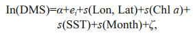 (1)
(1)where α was a grand mean, ei was a random intercept, s(·) was a one-dimensional nonlinear function based on a thin plate regression spline, and ζ was the residuals of the model. The spatial effects on the residuals were considered. The relationships between DMS and Chl a, and between DMS and SST, are shown in Fig. 2. Chl a was significantly correlated with DMS when Chl a was greater than 0.3 μg/L (P < 0.05). DMS increased with SST when SST was less than 22 C, but remained stable at SSTs above 22 ℃.

|
| Fig.2 Estimated smoothing curves for Chl a (a) and SST (b) The solid line is the smoother and the dotted lines are 95% point-wise confidence bands. |
After we established the GAMM, the correlations between all the in-situ DMS data and the simulated DMS data were determined. The correlation coefficient between these two datasets was 0.68 (Fig. 3a). To more precisely evaluate our model, we separated the spatial data into four subregions, divided by 40-m isobaths. We found that the in-situ and simulated data were well-correlated in coastal areas than in central areas: the correlation coefficient in the coastal YS was 0.70, while the correlation coefficient in the central YS was 0.62. Similarly, the correlation coefficient of the coastal ECS (0.71) was greater than that of mid-shelf ECS (0.63). This indicated that our GAMM simulated DMS more accurately in coastal areas, and that the correlation with observed data was acceptable in the YS. To further assess the reliability of the model, external validation was performed using the DMS data collected in 2015; this dataset included 186 data points collected over three seasons (spring, summer, and autumn) in the ECS. The correlation coefficient for this external validation dataset was 0.62.

|
| Fig.3 Validation in the East China Sea a. correlation between the in-situ observed DMS data and the simulated DMS data across all data points; b–e. correlations in four depth subregions. b. coastal YS; c. central YS; d. coastal ECS; e. mid-shelf ECS; f. external validation in 2015. |
Using our GAMM, we performed a 22-year surface seawater DMS concertation hindcast based on daily satellite SST and Chl-a data, with a spatial grid resolution unified to 1/4°.
2.3 DMS reconstructionDue to clouds, rain, or malfunctions, satellite images have gaps. To fill these missing data in our 22-year DMS concentrations, we used the Data Interpolation Empirical Orthogonal Function (DINEOF) method (Beckers and Rixen, 2003; Alvera-Azcárate et al., 2005; Beckers et al., 2006). The DINEOF is a self-consistent, parameter-free EOF-based method for gappy data fields, especially for large data matrices with many gaps.
After DINEOF reconstruction of the period 1998–2019, the time series for the monthly percentage anomalies in DMS, Chl-a, and SST levels were obtained as follows:
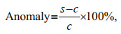 (2)
(2)where s was the monthly mean value and c was corresponding monthly climatological value derived by averaging the values for each month over the period 1998-2019.
To clearly demonstrate the interannual variation in DMS, a 24-month low-pass filter was applied to remove seasonal signals. Here the low-pass filter was used to pass signals with low frequency as well as block with high frequency than a preferred cut-off frequency. The standard deviation of the 22-year monthly mean DMS concentrations was used as a proxy for the amplitude of interannual variation. A linear regression of time series of the monthly mean DMS variation was calculated; the slope and intercept of the best fit line were calculated using the least squares method. To determine the point at which the linear relationship changed abruptly, the cumulative DMS departure from the mean DMS anomaly was used to delineate trends in DMS variation. Periodogram analysis (Bisina and Azeez, 2017) was used to determine the periodicity of the interannual DMS variation. Finally, the power spectral density was estimated by performing a Fast Fourier Transformation (FFT) on the sampled data.
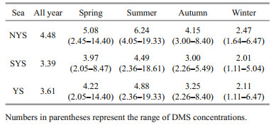
3 RESULT 3.1 Spatial and seasonal variations in DMS concentrationsThe annual mean concentration of surface seawater DMS in the YS was 3.61 nmol/L during the period 1998–2019. The average DMS concentrations in the North Yellow Sea (NYS) and the South Yellow Sea (SYS) were 4.48 and 3.39 nmol/L, respectively. Over the same period (1998–2019), the annual mean DMS concentration in the YS was 3.64 nmol/L. This is higher than the global annual mean DMS sea surface concentration for 1998–2017 (2.26 nmol/L; Lana et al., 2011).
The average DMS concentrations in the spring (Mar.–May), summer (Jun.–Aug.), autumn (Sep.–Nov.), and winter (Dec.–Feb.) were 4.22, 4.88, 3.25, and 2.11 nmol/L, respectively (Table 1). The seasonal and spatial distributions of DMS in the YS, based on monthly mean surface seawater values, are shown in Fig. 4. There were significant seasonal variations in DMS, with the highest DMS concentrations appearing in the summer, followed by spring, autumn, and winter. Across all seasons, DMS concentrations were greatest in the coastal waters of the NYS coastal water. The maximum DMS concentrations in the nearshore NYS in spring, summer, autumn, and winter were 14.40, 19.33, 8.40, and 6.47 nmol/L, respectively. On average, DMS concentrations were lowest in the southern SYS; DMS concentrations in the southern SYS in spring, summer, autumn, and winter were 2.05, 2.36, 2.26, and 1.11 nmol/L, respectively. The maximum standard deviation of mean nearshore DMS concentration was 5.86 nmol/L, which was greater than the minimum standard deviation in the SYS (0.14 nmol/L). In summary, the seasonal variations in surface seawater DMS concentration were greater in coastal waters than in offshore areas.

|
| Fig.4 Seasonal distributions of surface seawater DMS concentration The contours represent the standard deviations of monthly mean DMS. |
The contours in Fig. 4 show the amplitudes of interannual variations in DMS. The amplitudes of interannual variations in DMS were generally greater in spring and summer, and lower in autumn and winter. The amplitudes in coastal waters were greater than those in offshore areas. The greatest interannual variations in amplitude were found along the coasts of the Shandong Peninsula, Subei Shoal, and NYS during the summer, and the lowest interannual variations in amplitude were found in the central YS during the autumn and winter. The long-term annual trends and anomalies of the annual DMS means for the period 1998–2019 are shown in Fig. 5a. Annual mean DMS increased significantly from 1998 to 2012, and then decreased between 2013 and 2019. This indicated that interannual DMS variability varied by region, and that trends in interannual DMS variability were not monotonic.

|
| Fig.5 Monthly percentage anomalies in DMS in the YS (a) and gridded turning points in DMS trends (b) Contours represent 50-m isobath in (b). The four subregions chosen are indicated with boxed letters: A, B, C, and D. |
The gridded turning point of the annual trends in DMS was calculated using cumulative departure (Fig. 5b). The results indicated that turning points differed significantly among regions. Monthly DMS trends changed in 2014 or 2015 in the NYS; in 2017 is the west coastal and central SYS; and in 2012 in Subei Shoal, the southern SYS and the coastal SYS.
To further clarify regional differences, four subregions were established to represent the different identified turning points in DMS trends: domain A was located in the NYS, domain B was located in the western SYS, domain C was located in the central SYS, and domain D was located in Subei Shoal. To obtain a long-term DMS time series without the interference of the seasonal signal, seasonal signals were removed by applying a 24-month low-pass filter to the mean DMS anomaly percentage. The interannual variations in DMS anomaly percentages in domains A, B, C, and D are shown in Fig. 6.

|
| Fig.6 Interannual variations in surface seawater DMS anomalies for four chosen domains in the YS a. NYS; b. western SYS; c. central SYS; d. Subei Shoal. The solid grey lines represent DMS anomalies. The solid black lines represent DMS anomalies after low-pass filtering with a cut-off frequency of 1/24. The dashed red lines represent DMS trends. The dashed green lines indicate trend turning points. |
Obvious turning points in DMS anomaly trends were observed between 1998 and 2019 in each of the four subregions, consistent with the analysis shown in Fig. 5b. In domain A, surface seawater DMS anomalies increased significantly until 2015 (a 10% increase from 1998 to 2015), and then remained stable. Similar results were observed in domain B, where DMS anomalies increased 10.46% between 1998 and 2015, but decreased after 2015. However, unlike the insignificant variation observed in domain A, the DMS anomalies in domain B decreased by approximately 2.69% between 2015 and 2019.
Domain C is the only subregion in which DMS anomalies increased both before and after the turning point (2017), although the increase became more gradual after than the increase in domain A and domain B. In this region, DMS increased 6.44% from 1998 to 2017. The DMS increase may have slowed due to the Yellow Sea Cold Water Mass in this subregion. Domain D in Subei Shoal exhibited the greatest increase in DMS (13.94%) before the turning point; after the turning point, DMS decreased by 4.74%.
All of the trends reported above were statistically significant at the 95% confidence level. Overall, the earlier the DMS-trend turning point occurred in a given YS domain, the faster the DMS concentration increased before the turning point.
Figure 7 shows DMS anomaly trends in the YS before and after each turning point. Based on the turning points in the YS, we subdivided the original DMS anomaly percentage time series into two phases exhibiting inverse trends. Prior to the turning point, DMS anomaly percentages were positive across the entire YS, signifying an upward trend (Fig. 7a). The subregions exhibiting larger increases were mainly located in the shallow regions of the YS, especially in Subei Shoal. Conversely, after the turning point, DMS anomaly percentages were negative over most of the YS (with the exception of the central YS), indicating a downward trend (Fig. 7b).

|
| Fig.7 Distributions of the long-term DMS anomaly trends before (a) and after (b) the turning point Shaded grey areas exhibited non-significant trends (P > 0.05). Contours indicate 50-m isobaths. |
To identify periodic patterns in the long-term series of DMS, Chl-a, and SST anomalies, spectrum analyses were performed to estimate the power spectra of the three time series in each of the four chosen domains. All monthly data were filtered with a 24- to 120-month band-pass filter prior to power-spectrum estimation. The power spectral densities reflected the frequencies of three time series, and decomposed the raw data into different frequencies (Fig. 8).

|
| Fig.8 Power spectra of interannual DMS, Chl-a, and SST anomalies in the four subregions a. NYS; b. western SYS; c. central SYS; d. Subei Shoal. The dashed curves indicate the standard red noise. Blue shaded regions indicate the interannual cycle periods of the three variables. Green shaded regions represent the interannual cycle periods of DMS and Chl a only. Red shaded regions represent the interannual cycle periods of DMS and SST only. |
In subregion A, the power spectra of the DMS and SST anomalies peaked at 31, 38, 88, and 106 months, while the power spectrum of the Chl-a anomalies peaked significantly at 33, 44, and 88 months. Similar results were observed in domains B and C. In domain A, DMS and SST exhibited similar patterns of interannual variability, with periods of 31, 38, and 88–106 months. However, the patterns of interannual variation in the Chl-a anomalies differed from those of DMS and SST in both subregions. Spectrum peaks were identified at 31, 48, and 88 months in subregion B, and there was a possible time lag of 2–4 months between Chl a and DMS.
In domain C (central SYS), the patterns of interannual variation in DMS and SST were similar to the 31- and 38-month periods observed in subregions A and B. However, the interannual variation period of DMS was much longer (106 months), and the power spectrum was non-significant. There were only two variation periods in Chl a, one of approximately 35 months and one of approximately 48 months.
For domain D (Subei Shoal), DMS and Chl a seemed to have similarly long periods of interannual variation. Two significant peaks were observed in the power spectra of both variables, one at 48 months (4 years) and a second at 75 months (6.25 years). The SST anomalies in domain D exhibited three periods of interannual variation: 31, 38, and 75 months.
4 DISCUSSIONThe seasonal and interannual variability in SST and Chl a in the four closed subregions will be discussed in the following subsections. By comparing interannual DMS patterns with those of these two key environmental variables, we will assess whether DMS trends and cycles in each subregion can be explained by changes in SST and Chl a.
4.1 Effects of Chl a on interannual variation in DMSFigure 9 shows the zone-averaged interannual variations in DMS, Chl-a, and SST anomaly percentages in the four subregions for the period 1998–2019. The long-term trends of the DMS and Chl-a anomalies were similar: both variables had the same turning point in subregions B, C, and D. In subregion A, the turning point of Chl a was two years before that of DMS. These results indicated that the interannual variability in Chl a had a greater influence on interannual trends in DMS than SST in the YS. Correlation analysis identified a significant positive correlation between DMS and Chl a over the long-term in all four subregions. The coefficients of determination (R2) were 0.72, 0.83, 0.67, and 0.94 in subregions A, B, C, and D, respectively. However, SST was poorly correlated with DMS in the YS. Previous studies have identified a significant correlation between DMS and phytoplankton biomass in the surface seawater of the YS. In addition, based on DMS and Chl-a measurements taken during a variety of cruises, several studies have reported statistically significant positive correlations between DMS and Chl a (Yang et al., 2009, 2011b, 2012, 2014, 2015).

|
| Fig.9 Anomalies in DMS, Chl a, and SST for four subregions in the YS after the application of a 24-month low-pass filter a. NYS; b. western SYS; c. central SYS; d. Subei Shoal. Dashed lines correspond to the turning points calculated using cumulative departure. |
During the period 1998–2019, Chl-a concentration increased until the turning point and then decreased (Fig. 9). This increase in Chl a from 1998 to 2012 was consistent with previous results (Yamaguchi et al., 2012; Liu and Wang, 2013). It has been argued that the spatio-temporal variability of Chl-a concentration in the surface layer is associated with nutrient levels (Wang and Jiao, 1999; Liu et al., 2013b). Both riverine inputs and atmospheric deposition strongly influence the biogeochemistry of nutrient species in coastal and shelf oceans (Zhang et al., 2007a). Previous studies have shown that dissolved inorganic nitrogen (DIN) and the N/P ratio along the western coast of domain A increased during the period 1998–2008 (Yang et al., 2018). In domain B, DIN and the N/P ratio also appeared to increase (Wei et al., 2015), concomitant with the increase in Chl-a levels. Due to the greater riverine input from the Guanhe River and Sheyang River in domain D, the DIN and N/P ratio along the Subei Shoal also increased between 1996 and 2014 (Li et al., 2017).
In domain C, the increased use of nitrogen fertilizers since 1998 might be partially responsible for an increase in riverine DIN inputs into the YS (Wu et al., 2019). As one of the essential nutrient sources for the central YS (Guo et al., 2006; Zhang et al., 2007b; Yang et al., 2011a; Li et al., 2017), the Kuroshio intrusion might have an important influence on the interannual variability of Chl a. The variability of Kuroshio onshore intrusion across 200-m isobaths is roughly congruent with the interannual variations in Chl-a concentration in the central YS (Liu et al., 2014, 2015).
In domains A and B, the period of interannual variability for Chl a and DMS was 88 months (about 7.3 years). Both variables exhibited 48-month (4-year) and 75-month (6.25-year) cycles in domain D. In domain C, Chl a and DMS both peaked at 106 months (about 8.8 years), although these peaks were not significant.
4.2 Effects of SST on the interannual variation in DMSSurface seawater DMS concentrations were regulated by a subtle dynamic equilibrium between the rates of DMS production and of DMS consumption. Some studies have shown that SST directly or indirectly physically influences DMS concentrations in the surface water. In addition, SST was the principal factor affecting the efficiency of zooplankton grazing, which might represent a potential DMS sink (Yu et al., 2015). Enzyme activity increases with strong zooplankton grazing, and this process affects the source of surface seawater DMS (Wolfe et al., 1997). By influencing bacterial activity, SST indirectly controls DMS consumption (Zhao, 2007).
SST exhibited similar interannual patterns across all four subregions: the SST anomaly decreased significantly between 1998 and 2012, and then increased from 2013 to 2019. These results indicated that DMS and SST were consistently correlated. In subregions A, B, and C, the interannual variations were shown to be 31 and 38 months (about 2.6 and 3.17 years, respectively) during the 1998–2019 period (Fig. 8). Additionally, longer periods of interannual variability were identified: 88–106 months in subregions A and B, 106 months in subregion C, and 75 months in subregion D. This may explain why SST is the main driver of interannual DMS variability over shorter timescales (2–3 years), while both SST and Chl a drive interannual DMS variability over longer timescales (7–8.8 years).
SST anomalies were strongly correlated with the meridional and zonal components of the winter monsoon in the YS during the period 1976–2008. The period of interannual variability of SST was 2–3 years. El Niño-Southern Oscillation (ENSO) events might affect wind fields in the YS, leading to alterations in the pathway and extent of the Yellow Sea Warm Current (Wang et al., 2008). The water temperature in section the Pollution Nagasaki (PN) section was influenced by the invasion of Kuroshio and was significantly correlated with the Pacific Decadal Oscillation index (Hu et al., 2018). Liu et al. (2013a) found that, between 1950 and 2007, patterns of interannual SST variability in the China Sea corresponded to the Niño-3 index, with correlations being the highest when a lag of 10 months was allowed in periods of 2–7 years. In addition, Wang et al. (2020) found that the periodicity of the interannual variability of the SST anomaly was about 2.5 years during the period 1985–2017; allowing a 6-month lag, this variation was well correlated with the Niño-3.4 index. Regular, periodic, strong Pacific ENSO events may regulate the interannual variability of SST in the YS (Zhang et al., 2009; Wang et al., 2020).
5 CONCLUSIONIn this study, the long-term (1998–2019) trends in surface seawater DMS concentrations in the YS were characterized using a continuous 22-year DMS dataset. This dataset was obtained using a DMS GAMM based on the historical in situ sampling, as well as satellite SST and modified Chl-a data.
The DMS concentration in YS surface seawater was 3.61 nmol/L. DMS concentrations in the spring and summer were significantly higher than those in the autumn and winter. In the YS, DMS values were highest nearshore and were generally lowest offshore. Beginning in 1998, DMS concentration increased significantly in the YS until the turning point. The earlier the turning point occurred, the more quickly DMS concentration increased before the transition and the greater the decrease after the transition. Chl a appears to be the main factor influencing interannual patterns of DMS in the YS. Interannual cycles of DMS were under the joint control of Chl a and SST: short-term variations in DMS (2–3 years) were strongly affected by SST, while longer term variations (6–8 years) were affected by both Chl a and SST. The variability in Chl a was mainly affected by anthropogenic eutrophication and natural processes, while SST was mainly associated with natural processes.
6 DATA AVAILABILITY STATEMENTThe data that support the findings of this study are available from the corresponding author upon reasonable request.
7 ACKNOWLEDGMENTThe authors are grateful to the captain and crew of the R/V Dong Fang Hong 2 for help and cooperation during the study. We are thankful to Dr. Qiang HAO (Second Institute of Oceanography, Ministry of Natural Resources, China) for providing locally modified chlorophyll dataset. We also wish to thank the colleagues in our laboratory for the discussion of this study.
Alvera-Azcárate A, Barth A, Rixen M, Beckers J M. 2005. Reconstruction of incomplete oceanographic data sets using empirical orthogonal functions: application to the Adriatic Sea surface temperature. Ocean Modelling, 9(4): 325-346.
DOI:10.1016/j.ocemod.2004.08.001 |
Andreae M O, Barnard W R. 1984. The marine chemistry of dimethylsulfide. Marine Chemistry, 14(3): 267-279.
DOI:10.1016/0304-4203(84)90047-1 |
Andreae M O, Ferek R J, Bermond F, Byrd K P, Engstrom R T, Hardin S, Houmer P D, Lemarrec F Raemdonck H, Chatfield R B. 1985. Dimethyl sulfide in the marine atmosphere. Journal of Geophysical Research: Atmospheres, 90(D7): 12891-12900.
DOI:10.1029/JD090iD07p12891 |
Andreae M O, Rosenfeld D. 2008. Aerosol-cloud-precipitation interactions. Part 1. The nature and sources of cloud-active aerosols. Earth-Science Reviews, 89(1-2): 13-41.
|
Andreae M O. 1986. The Ocean as a Source of Atmospheric Sulfur Compounds. In: Buat-Ménard P ed. The Role of Air-Sea Exchange in Geochemical Cycling. Springer, Dordrecht. p. 331-362.
|
Andreae M O. 1990. Ocean-atmosphere interactions in the global biogeochemical sulfur cycle. Marine Chemistry, 30: 1-29.
DOI:10.1016/0304-4203(90)90059-L |
Beckers J M, Barth A, Alvera-Azcárate A. 2006. DINEOF reconstruction of clouded images including error maps—application to the sea-surface temperature around Corsican Island. Ocean Science Journal, 2(2): 183-199.
DOI:10.5194/os-2-183-2006 |
Beckers J M, Rixen M. 2003. EOF calculations and data filling from incomplete oceanographic datasets. Journal of Atmospheric and Oceanic Technology, 20(12): 1839-1856.
DOI:10.1175/1520-0426(2003)020<1839:ECADFF>2.0.CO;2 |
Bisina K V, Azeez M A. 2017. Optimized estimation of power spectral density. In: 2017 International Conference on Intelligent Computing and Control Systems (ICICCS). IEEE, Madurai. p. 871-875.
|
Charlson R J, Lovelock J E, Andreae M O, Warren S G. 1987. Oceanic phytoplankton, atmospheric sulphur, cloud albedo and climate. Nature, 326(6114): 665-661.
|
Guo X Y, Miyazawa Y, Yamagata T. 2006. The Kuroshio onshore intrusion along the shelf break of the East China Sea: the origin of the Tsushima Warm Current. Journal of Physical Oceanography, 36(12): 2205-2231.
DOI:10.1175/JPO2976.1 |
Gypens N, Borges A V. 2014. Increase in dimethylsulfide (DMS) emissions due to eutrophication of coastal waters offsets their reduction due to ocean acidification. Frontiers in Marine Science, 1: 4.
|
Hao Q, Chai F, Xiu P, Bai Y, Chen J F, Liu C G, Le F F, Zhou F. 2019. Spatial and temporal variation in chlorophyll a concentration in the Eastern China Seas based on a locally modified satellite dataset. Estuarine, Coastal and Shelf Science, 220: 220-231.
DOI:10.1016/j.ecss.2019.01.004 |
Houghton J T. 2001. Intergovernmental Panel on Climate Change (IPCC). Cambridge Univ. Press, New York. p.881.
|
Hu Y Y, Guo X Y, Zhao L. 2018. Interannual variation of nutrients along a transect across the Kuroshio and shelf area in the East China Sea over 40 years. Journal of Oceanology and Limnology, 36(1): 62-76.
DOI:10.1007/s00343-017-6234-y |
Jian S, Zhang H H, Zhang J, Yang G P. 2018. Spatiotemporal distribution characteristics and environmental control factors of biogenic dimethylated sulfur compounds in the East China Sea during spring and autumn. Limnology and Oceanography, 63(S1): S280-S298.
DOI:10.1002/lno.10737 |
Kloster S, Six K D, Feichter J, Maier-Reimer E, Roeckner E, Wetzel P, Stier P, Esch M. 2007. Response of dimethylsulfide (DMS) in the ocean and atmosphere to global warming. Journal of Geophysical Research: Biogeosciences, 112(G3): G03005.
|
Lana A, Bell T G, Simó R, Vallina S M, Ballabrera-Poy J, Kettle A J, Dachs J, Bopp L, Saltzman E S, Stefels J, Johnson J E, Liss P S. 2011. An updated climatology of surface dimethlysulfide concentrations and emission fluxes in the global ocean. Global Biogeochemical Cycles, 25(1): GB1004.
|
Li C X, Yang G P, Wang B D, Xu Z J. 2016. Vernal distribution and turnover of dimethylsulfide (DMS) in the surface water of the Yellow Sea. Journal of Geophysical Research: Oceans, 121(10): 7495-7516.
DOI:10.1002/2016JC011901 |
Li H M, Zhang Y Y, Tang H J, Shi X Y, Rivkin R B, Legendre L. 2017. Spatiotemporal variations of inorganic nutrients along the Jiangsu coast, China, and the occurrence of macroalgal blooms (green tides) in the southern Yellow Sea. Harmful Algae, 63: 164-172.
DOI:10.1016/j.hal.2017.02.006 |
Liu C Y, Wang F, Chen X P, von Storch J S. 2014. Interannual variability of the Kuroshio onshore intrusion along the East China Sea shelf break: effect of the Kuroshio volume transport. Journal of Geophysical Research: Oceans, 119(9): 6190-6209.
DOI:10.1002/2013JC009653 |
Liu D Y, Wang Y Q. 2013. Trends of satellite derived chlorophyll-a (1997-2011) in the Bohai and Yellow Seas, China: effects of bathymetry on seasonal and inter-annual patterns. Progress in Oceanography, 116: 154-166.
DOI:10.1016/j.pocean.2013.07.003 |
Liu N, Wang H, Ling T J, Feng L C. 2013a. The influence of ENSO on sea surface temperature variations in the China seas. Acta Oceanologica Sinica, 32(9): 21-29.
DOI:10.1007/s13131-013-0348-7 |
Liu X, Chiang K P, Liu S M, Wei H, Zhao Y, Huang B Q. 2015. Influence of the Yellow Sea Warm Current on phytoplankton community in the central Yellow Sea. Deep Sea Research Part Ⅰ: Oceanographic Research Papers, 106: 17-29.
DOI:10.1016/j.dsr.2015.09.008 |
Liu Y, Zhang T R, Shi J H, Gao H W, Yao X H. 2013b. Responses of chlorophyll a to added nutrients, Asian dust, and rainwater in an oligotrophic zone of the Yellow Sea: Implications for promotion and inhibition effects in an incubation experiment. Journal of Geophysical Research: Biogeosciences, 118(4): 1763-1772.
DOI:10.1002/2013JG002329 |
Lovelock J E, Maggs R J, Rasmussen R A. 1972. Atmospheric dimethyl sulphide and the natural sulphur cycle. Nature, 237(5356): 452-453.
DOI:10.1038/237452a0 |
Nguyen B C, Mihalopoulos N, Putaud J P, Gaudry A, Gallet L, Keene W C, Galloway J N. 1992. Covariations in oceanic dimethyl sulfide, its oxidation products and rain acidity at Amsterdam Island in the Southern Indian Ocean. Journal of Atmospheric Chemistry, 15(1): 39-53.
DOI:10.1007/BF00053608 |
Qu B, Yang G P, Guo L Y, Zhao L. 2020a. The satellite derived environmental factors and their relationships with dimethylsulfide in the east marginal seas of China. Journal of Marine Systems, 204: 103305.
DOI:10.1016/j.jmarsys.2020.103305 |
Qu B, Zhao L, Gabric A J. 2020b. Simulating the sea-to-air flux of dimethylsulfide in the eastern China marginal seas. Journal of Marine Systems, 212: 103450.
DOI:10.1016/j.jmarsys.2020.103450 |
Sciare J, Mihalopoulos N, Nguyen B C. 2002. Spatial and temporal variability of dissolved sulfur compounds in European estuaries. Biogeochemistry, 59(1-2): 121-141.
|
Six K D, Kloster S, Ilyina T, Archer S D, Zhang K, Maier-Reimer E. 2013. Global warming amplified by reduced sulphur fluxes as a result of ocean acidification. Nature Climate Change, 3(11): 975-978.
DOI:10.1038/nclimate1981 |
Song S K, Shon Z H, Choi Y N, Son Y B, Kang M, Han S B, Bae M S. 2019. Global trend analysis in primary and secondary production of marine aerosol and aerosol optical depth during 2000-2015. Chemosphere, 224: 417-427.
DOI:10.1016/j.chemosphere.2019.02.152 |
Uher G. 2006. Distribution and air-sea exchange of reduced sulphur gases in European coastal waters. Estuarine, Coastal and Shelf Science, 70(3): 338-360.
DOI:10.1016/j.ecss.2006.05.050 |
Wang H W, Yu F, G. L L, Diao X Y, Guo J S. 2008. Characteristics of spatial and interannual variation in the Yellow Sea Warm Current area in winter. Advances in Marine Science, 27(2): 140-148.
(in Chinese with English abstract) |
Wang M, Guo J R, Song J, Fu Y Z, Sui W Y, Li Y Q, Zhu Z M, Li S, Li L L, Guo X F, Zuo W T. 2020. The correlation between ENSO events and sea surface temperature anomaly in the Bohai Sea and Yellow Sea. Regional Studies in Marine Science, 35: 101228.
DOI:10.1016/j.rsma.2020.101228 |
Wang Y, Jiao N Z. 1999. The primary research of nutrient limitation of phytoplankton in northern Yellow Sea. Oceanologia et Limnologia Sinica, 30(5): 512-518.
(in Chinese with English abstract) |
Wei Q S, Yao Q Z, Wang B D, Wang H W, Yu Z G. 2015. Long-term variation of nutrients in the southern Yellow Sea. Continental Shelf Research, 111: 184-196.
DOI:10.1016/j.csr.2015.08.003 |
Wolfe G V, Steinke M, Kirst G O. 1997. Grazing-activated chemical defence in a unicellular marine alga. Nature, 387(6636): 894-897.
DOI:10.1038/43168 |
Wood S N. 2017. Generalized Additive Models: an Introduction with R. 2nd edn. CRC Press, Portland. p.496.
|
Wu G J, Cao W Z, Wang F F, Su X L, Yan Y Y, Guan Q S. 2019. Riverine nutrient fluxes and environmental effects on China's estuaries. Science of the Total Environment, 661: 130-137.
DOI:10.1016/j.scitotenv.2019.01.120 |
Xu F, Jin N, Ma Z, Zhang H H, Yang G P. 2019. Distribution, occurrence, and fate of biogenic dimethylated sulfur compounds in the Yellow Sea and Bohai Sea during spring. Journal of Geophysical Research: Oceans, 124(8): 5787-5800.
DOI:10.1029/2019JC015085 |
Yamaguchi H, Kim H C, Son Y B, Kim S W, Okamura K, Kiyomoto Y, Ishizaka J. 2012. Seasonal and summer interannual variations of SeaWiFS chlorophyll a in the Yellow Sea and East China Sea. Progress in Oceanography, 105: 22-29.
DOI:10.1016/j.pocean.2012.04.004 |
Yang D Z, Yin B S, Liu Z L, Feng X R. 2011a. Numerical study of the ocean circulation on the East China Sea shelf and a Kuroshio bottom branch northeast of Taiwan in summer. Journal of Geophysical Research: Oceans, 116(C5): C05015.
|
Yang F X, Wei Q S, Chen H T, Yao Q Z. 2018. Long-term variations and influence factors of nutrients in the western North Yellow Sea, China. Marine Pollution Bulletin, 135: 1026-1034.
DOI:10.1016/j.marpolbul.2018.08.034 |
Yang G P, Song Y Z, Zhang H H, Li C X, Wu G W. 2014. Seasonal variation and biogeochemical cycling of dimethylsulfide (DMS) and dimethylsulfoniopropionate (DMSP) in the Yellow Sea and Bohai Sea. Journal of Geophysical Research: Oceans, 119(12): 8897-8915.
DOI:10.1002/2014JC010373 |
Yang G P, Zhang H H, Su L P, Zhou L M. 2009. Biogenic emission of dimethylsulfide (DMS) from the North Yellow Sea, China and its contribution to sulfate in aerosol during summer. Atmospheric Environment, 43(13): 2196-2203.
DOI:10.1016/j.atmosenv.2009.01.011 |
Yang G P, Zhang H H, Zhou L M, Yang J. 2011b. Temporal and spatial variations of dimethylsulfide (DMS) and dimethylsulfoniopropionate (DMSP) in the East China Sea and the Yellow Sea. Continental Shelf Research, 31(13): 1325-1335.
DOI:10.1016/j.csr.2011.05.001 |
Yang G P, Zhang J W, Li L, Qi J L. 2000. Dimethylsulfide in the surface water of the East China Sea. Continental Shelf Research, 20(1): 69-82.
DOI:10.1016/S0278-4343(99)00039-4 |
Yang G P, Zhuang G C, Zhang H H, Dong Y, Yang J. 2012. Distribution of dimethylsulfide and dimethylsulfoniopropionate in the Yellow Sea and the East China Sea during spring: spatio-temporal variability and controlling factors. Marine Chemistry, 138-139: 21-31.
DOI:10.1016/j.marchem.2012.05.003 |
Yang J, Yang G P, Zhang H H, Zhang S H. 2015. Spatial distribution of dimethylsulfide and dimethylsulfoniopropionate in the Yellow Sea and Bohai Sea during summer. Chinese Journal of Oceanology and Limnology, 33(4): 1020-1038.
DOI:10.1007/s00343-015-4188-5 |
Yu J, Tian J Y, Yang G P. 2015. Effects of Harpacticus sp. (Harpacticoida, copepod) grazing on dimethylsulfoniopropionate and dimethylsulfide concentrations in seawater. Journal of Sea Research, 99: 17-25.
DOI:10.1016/j.seares.2015.01.004 |
Zhang G S, Zhang J, Liu S M. 2007a. Characterization of nutrients in the atmospheric wet and dry deposition observed at the two monitoring sites over Yellow Sea and East China Sea. Journal of Atmospheric Chemistry, 57(1): 41-57.
DOI:10.1007/s10874-007-9060-3 |
Zhang J, Liu S M, Ren J L, Zhang G L. 2007b. Nutrient gradients from the eutrophic Changjiang (Yangtze River) Estuary to the oligotrophic Kuroshio waters and reevaluation of budgets for the East China Sea Shelf. Progress in Oceanography, 74(4): 449-478.
|
Zhang S, Yu F, Diao X Y, Guo J S. 2009. The characteristic analysis on sea surface temperature inter-annual variation in the Bohai Sea, Yellow Sea and East China Sea. Marine Sciences, 33(8): 76-81.
(in Chinese with English abstract) |
Zhao S J. 2007. The ecological study of the picoplankton in the East China Sea and the Yellow Sea. Ocean University of China, Qingdao. (in Chinese)
|