 2022, Vol. 40
Institute of Oceanology, Chinese Academy of Sciences
Article Information
- SHA Jin, LI Xiaoming, YAN Xiaohai
- Relative contributions of temperature and salinity to steric sea level over the South China Sea
- Journal of Oceanology and Limnology, 40(2): 428-437
- http://dx.doi.org/10.1007/s00343-021-1057-2
Article History
- Received Feb. 16, 2021
- accepted in principle Mar. 16, 2021
- accepted for publication Apr. 13, 2022


2 Hainan Key Laboratory of Earth Observation, Sanya 502022, China;
3 Center for Remote Sensing, College of Earth, Ocean and Environment, University of Delaware, Newark 19711, DE, USA;
4 Joint Institute for Coastal Research and Management, University of Delaware/Xiamen University, USA/China
The South China Sea (SCS) is a semiclosed marginal sea to the southwest of the North Pacific Ocean, spanning from the Equator to approximately 23°N (Fig. 1). Numerous literatures have documented the hydrographic differences between the northern and southern SCS. In the northern SCS (NSCS), the Kuroshio intrusion and the SCS warm current (Hu et al., 2000; Xue et al., 2004) could mix the North Pacific Tropical Water (NPTW) and North Pacific Intermediate Water (NPIW) (Qu et al., 2000) with local SCS water masses (Zeng et al., 2016). In the southern SCS (SSCS), the seawater is recognized as part of the Indo-Pacific Warm Pool (IPWP), characterized by the accumulation of constant warm waters >28 ℃ (Yan et al., 1992; Weller et al., 2016). The lack of seasonality of the IPWP surface water temperature with seasonally varying surface salinity (De Deckker, 2016) in the SSCS can generate environmental impacts that are in contrast with the NSCS, including steric sea level variability.

|
| Fig.1 The bathymetry of the study area The shaded rectangle (114°N±1°) represents the transection analyzed later. |
Steric sea level corresponds to seawater volume expansion due to density variation from varying temperatures and salinities and is an essential component of sea level variation (Gill and Niller, 1973). The steric components are a significant contribution to the SCS deep basin (Cheng and Qi, 2010; Wu et al., 2017), and may be the major cause of the SCS interannual sea level variability (Feng et al., 2012). The documented hydrographic conditions between the NSCS and SSCS correspond to different characteristics of seawater density variations, and thus could naturally result in varying relative contributions of temperature and salinity to the steric height (i.e., the constitution of the steric sea level), which, however, is not well documented in the SCS. The steric sea level constitution could be particularly essential in ocean heat storage estimation based on altimetry (Chambers et al., 1997; Yan et al., 2004), as well as remote sensing applications of subsurface processes (Yan et al., 2006; Sha et al., 2015; Belonenko and Fedorov, 2018; Su et al., 2020), thus requires detailed clarification.
Moreover, the contribution of salinity to steric height is usually neglected when thermosteric height dominates but may be subject to regional differences as documented regarding Pacific Ocean sea-level variability (Wu et al., 2017). The development of sea surface salinity (SSS) remote sensing monitoring shows promising results in capturing SSS variability (Klemas, 2011), such as the ongoing salinification in the SCS in recent years (Zeng et al., 2018). Taking advantage of satellite observations at the mesoscale to conduct a comparison between the thermal- and halosteric components in the SCS is of specific scientific interest.
This study evaluates the meridional steric sea level constitution transition in the SCS. To achieve this goal, we define a contribution factor based on satellite datasets in Section 2. The steric constitutions for both the surface and interior of the ocean are presented in Section 3, and relative driving forces are diagnosed in Section 4. Discussion, summary, and conclusion are given in Sections 5 and 6.
2 DATA AND METHOD 2.1 DatasetTo investigate the SCS sea surface temperature (SST) variability, we use the daily product of the microwave and infrared optimal interpolated SST (MW-IR OISST) provided by Remote Sensing Systems (RSS). The product combines both microwave and infrared SST measurements at the global scale with a spatial resolution of 9 km spanning from 2002 to the present. The data are part of the Global Ocean Data Assimilation Experiment (GODAE) High-Resolution SST Pilot Project (GHRSST-PP) with a diurnal model to create a foundation SST.
The sea surface salinity (SSS) data are from the Soil Moisture Active Passive (SMAP) SSS V4.0 validated release from RSS. The SMAP was launched in 2015, using an L-band passive radiometer to measure SSS and sea surface wind speed. The data are the L3 daily product with 8-day running averages and a spatial resolution of 70 km spanning from 2015 to the present. A triple collocation validation with monthly SMAP V3, Argo data, and HYCOM simulation (Meissner et al., 2019) revealed that the standard deviation of the SMAP data is less than 0.2. The SST anomaly (SSTA) and SSS anomaly (SSSA) are also used in this study to investigate the steric variability (see Section 2.2), which are calculated with reference to the mean from January of 2015 to December of 2019.
Other datasets are also used to achieve the research goals. Air-sea heat flux terms including surface latent heat flux (LHF), surface sensible heat flux (SHF), surface solar radiation (SSR), and surface thermal radiation (STR) are available from ERA5 (Hersbach et al., 2019), which is the fifth generation European Centre for Medium-Range Weather Forecasts (ECMWF) atmospheric reanalysis of the global climate with a 0.25° grid size and a 6-hour temporal resolution. The ERA5 air-sea heat flux components were evaluated recently in the Arabian Gulf and Red Sea with biases of 4.5 W/m2 and 1.59 W/m2, respectively (Al Senafi et al., 2019). The sea surface wind stress, precipitation, and evaporation data also come from the ERA5 reanalysis. Sea Level Anomaly (SLA) data could be accessed from the European Copernicus Marine Environment Monitoring Service (CMEMS) that is a reprocessed global multisensormerged L4 product as previously delivered by AVISO+ with a spatial resolution of 0.25° on a daily basis. For the interior of the ocean, we use the Simple Ocean Data Assimilation ocean/sea-ice reanalysis (SODA, version 3.4.2) (Carton et al., 2018) with a spatial resolution of 0.25° and 50 vertical levels (the vertical starting depth is 7 m). The vertical resolution is linearly interpolated to 1 m. Comparisons among different datasets (e.g. Belonenko and Koldunov, 2019; Carton et al., 2019) have validated the application of SODA in sea level studies.
To utilize these multisensor datasets, all variables are interpolated into a grid of 0.125° following Sha et al. (2017) to maintain data coverage to the best extent in calculation procedures such as gradient estimation while coordinating the varying resolutions of datasets ranging from 9 km to 70 km. We choose 105°E–122°E, 5°N–24°N as our study area, and 2015 to 2019 as our study period.
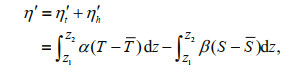
2.2 Estimation of steric componentsThe steric height is an important component of sea level variation, representing variations of the water volume given no water mass changed. The total steric height can be further decomposed into thermal steric height (TS) and haline steric height (HS), corresponding to the variation in seawater temperature and salinity respectively. Following previous documents (e.g., Gill and Niller, 1973; Sha et al., 2015), the thermal and haline steric components are estimated as
 (1)
(1) (2)
(2)where T and S represent the seawater temperature and salinity, respectively, while T S and are the temporal means. Z1 and Z2 are the integration depths. α and β are the thermal expansion coefficient and haline contraction coefficient respectively. ρ0 is a representative surface density constant.
In a common steric height estimation procedure, Z1 is chosen to be an assumed level of no motion, 1 000 m for example, and Z2 is chosen as 0 m. In our specific steric estimation procedures, temperature and salinity profiles from SODA are first converted into conservative temperature Θ and absolute salinity SA following TEOS-10 as Θ is more conservative than the potential temperature and SA provides the best mass fraction estimate of the dissolved matter. Since SODA profiles start at 7 m, we then calculate the thermal and haline steric components within each 1-m depth interval from 7 m to 1 000 m (or the water bottom for shallower regions). The total integrated steric height needs no further calculation so that we can focus on the steric constitution within each 1-m layer while avoiding additional approximation of the upper 7 m.
Concerning the integration depth, the contribution of the surface layer to the whole volume steric height might be small. However, the surface layer has the largest spatial-temporal variability. As shown in Fig. 2, the domain-averaged standard deviations (STDs) of the temperature/salinity anomaly, as well as the derived TS and HS are estimated based on SODA data. These STDs decrease more than one order of magnitude from the surface (or more accurately, 7 m) to 1 000-m depth. This is because most dynamic activities occur in the ocean surface layer, where the atmosphere and the ocean interact with each other with freshwater and heat exchanges. Hence, it is necessary and meaningful to first clarify the steric variability of the surface layer. The so-called "surface steric height" is thus calculated in this study by integrating within the upper unit meter using SST and SSS from satellite observations. Then, TS and HS are compared with each other. The investigation of this very thin slab could well represent the ocean upper mixed layer while avoiding uncertainties introduced by the mixed layer depth estimation, and could help to describe the steric constitution over the atmosphere-ocean interface.

|
| Fig.2 Vertical distributions of seawater temperature and salinity STDs averaged over SCS a. temperature (red) and salinity (black) anomalies with the temporal mean (from 2015 to 2019) removed; b. thermal (red, TS) and haline (black, HS) steric components at each depth level. The calculation is based on SODA data. |
To quantify the relative contributions of salinity and temperature to the temporal oscillation of sealevel variability, we define the contribution factors CFH for salinity and CFT for temperature in this study as
 (3)
(3) (4)
(4)where σ2 represents the variance of steric heights calculated along the temporal dimension for TS and HS (Section 2.2). Since the steric height components are all perturbations around the level of zero, we use ratios based on STD rather than direct magnitude ratios between TS and HS to avoid extrema induced by cross-zero points of steric height values. By definition, CFs are nondimensional, and
 (5)
(5)For example, in the case of TS and HS having the same standard deviation (STD), CFH≈0.70; if TS STD is twice as much as the HS STD, CFH≈0.45.
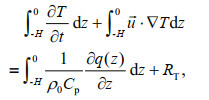
2.4 Surface temperature and salinity balancesThe upper layer heat balance equation (Stevenson and Niiler, 1983) could be simplified as
 (6)
(6) (7)
(7)where T is the seawater temperature, 
Similarly, the surface layer seawater salinity balance equation (Delcroix and Hénin, 1991) can be expressed as
 (8)
(8) (9)
(9)where S is the seawater salinity, and F is the vertical salt flux in units of m/s. H is set to be 1 m in calculations. S0 denotes the salinity at the top of the layer. Over the surface, F(0) represents the dilution effect of the surface volume due to precipitation (P) and evaporation (E). RS is the residual term indicating factors such as entrainment mixing.
Since we intend to evaluate the roles of driving forces in the surface and upper layer steric sea level variability, no attempt is made to construct complete heat and salt balances. Additionally, the framework of horizontal advection estimation (Sha et al., 2017, 2019) is employed to estimate the surface layer advection, with geostrophic and Ekman currents estimated from the SLA and wind stress (Welander, 1957), while SST and SSS are used as the upper layer temperature and salinity.
3 STERIC CONSTITUTIONS IN THE SCS 3.1 Surface layerBased on the variance of the SSTA and SSSA, the relative contributions of temperature and salinity to the total steric variation could be well quantified by CFH (Fig. 3). One major feature is the increasing contribution of the haline steric from the northern basin to the southwest SCS. For the deep basin areas between 15°N–22°N, the CFH is less than 0.45, suggesting that TS has at least twice the STD than HS. Over the southeastern part of the SCS, CFH is in the range of 0.7–0.9, thereby representing a larger variability in HS relative to TS. High CFH areas are also observed near the estuary of the Zhujiang (Pearl) River and Mekong River (Su, 2004) but are confined within the shelf. The southeastern high CFH area shows a coherent pattern with the Sulu Sea across Palawan Island. Isolines are also generally inclined in the northeast-southwest direction, suggesting a possible connection with the SCS circulation (Liu et al., 2001; De Deckker, 2016). It is also worth mentioning that the smallest CF value is 0.31, locating at approximately 17°N/112°E. In other words, there is no area where TS STDs are one order larger than those of HS, thus the salinity variability could not be neglected in the SCS steric sea level estimation.

|
| Fig.3 CFH over SCS surface layer Black lines indicate the isolines of 0.45 and 0.70 as mentioned in Section 2.3. |
A meridional transection along 114°E (Fig. 1), which is approximately in the middle of the SCS basin, is investigated for different variables to clarify the meridional CFH transition. Ambient areas spanning from 113°E to 115°E are also included to reduce the noise (Fig. 4). Consistent with Fig. 3, steric sea level variability is dominated by TS between 9°N and 21°N, with the dominant role switching to HS gradually from 9°N to the south. The distribution of CFs depends on the distribution of both TS and HS: TS STDs decrease almost monotonically southward between 21°N and 8°N, while HS STDs are large over the northern SCS shelf, low in the deep basin, and increase southward.

|
| Fig.4 CFs and temporal STD of steric height components along the 114ºE transection Blue lines are HS, and red lines are TS. The error bars indicate the spatial STD across 113°E and 115°E. |
SODA data are used to investigate the vertical distribution of the relative contributions of temperature and salinity. First, the surface layer CFH from SODA (Fig. 5) is generally consistent with that from satellite observations (Figs. 3 & 4). The CFH pattern is coherently extended to approximately 50-m depth where CFH reduces to less than 0.4. From the depth underneath, TS plays the dominant role. Wu et al. (2017) suggested that temperature variability could peak approximately 100 m while salinity is surfaceintensified concerning interannual and decadal time scales over the Indo-Pacific region. Our results based on SODA profiles reveal that a similar distribution holds for the temporal variability over the SCS regional scale.

|
| Fig.5 Vertical extension of the CFH along 114°E based on SODA profiles |
Consistent distributions of the steric constitution are revealed in the above analysis for both the surface steric height based on satellite observations and the upper 50 m based on SODA data. To clarify the involved driving forces, we hereby focus our analysis over the surface ocean and consider impacts from two perspectives: the surface heat/freshwater flux and the horizontal heat/salt advection. Since the steric height is induced by anomalous T/S variability, the STDs of each variable are compared rather than the long-term mean. In total, four variables are evaluated along the same 114°E transection: surface horizontal salt advection (Fig. 6a), surface horizontal heat advection (Fig. 6b), surface freshwater input F(0) as in Eq.9 (Fig. 6c), and surface heat flux q(0) as in Eq.7 (Fig. 6d). It should be noted that the surface freshwater flux, including precipitation and evaporation, could influence sea level by changing both the water mass distribution and steric height variations. Here we only consider the relation between the freshwater flux and the steric height while leaving the mass effect for future investigations.

|
| Fig.6 STD of driving factors along the transection a. surface salt advection STD; b. surface heat advection; c. surface salt flux; d. surface heat flux. |
Salinity advection varies mostly over the northern and southern marginal regions which are close to the continent. The heat advection also peaks over the northern continental shelf and oscillates across the deep basin. Different distribution patterns are found for both the freshwater input and heat flux. Variations in the surface freshwater input focus on the northern continental shelf 16°N–22°N and regions between 7°N–14°N, while the heat flux coherently decreases from north to south, which is consistent with the TS STD.
Further diagnostics are also conducted to distinguish detailed driving factors (Fig. 7): the heat/ salt advection could be decomposed into the geostrophic advection driven by the barotropic geostrophic currents and the Ekman advection driven by the wind stress curl; the surface freshwater input could be separated into evaporation and precipitation; and the surface heat flux consists of LHF, SHF, SSR, and STR as introduced in Section 2.4. Concerning the north-south imbalance and temporal variability, the geostrophic current, for both salt and heat, is the dominant driving factor within the advection. For the surface freshwater input, variation in precipitation is the dominant factor. It should also be noted that Fig. 7c indicates a direct comparison between evaporation and precipitation, and thus is one order smaller than the salt flux term (Fig. 6c) as expected by recalling Eq.9. For the heat flux, the STDs of the LHF and SSR are much larger than those of the SHF and STR, while the LHF STDs show an apparent north-south inclining trend that is consistent with the inclined SSTA STD.

|
| Fig.7 Diagnostics of the driving forces STDs along the 114°E transect a. Ekman and geostrophic salt advection; b. Ekman and geostrophic heat advection; c. precipitation (P) and evaporation (E) in the surface freshwater input; d. LHF, SHF, SSR, and STR in the surface heat flux. |
As analyzed above, the steric constitution, i.e., the relative contributions of temperature and salinity to the steric sea level, is investigated using satellite observations and SODA data. The southward-decreasing thermosteric height variability is most likely related to the reduced heat flux variation southward, especially the southward reducing LHF. For those of the haline steric height, the increased variation over the northern and southern SCS continental shelf comes from the strong geostrophic salinity advection, while the reduced precipitation variability contributes to the depressed HS variability in the central SCS deep basin.
Scale analysis could be conducted on magnitudes of driving forces (Fig. 6). For the salinity variation, both advection and surface salt flux are in units of m/s, and are both on the same order of magnitude (10-6 m/s), indicating a combined impact of salt advection and surface flux on the halosteric variability across the SCS. This is consistent with early studies confirming the roles of rainfall and salt advection over the tropical Pacific (Delcroix and Hénin, 1991; Cronin and McPhaden, 1998) and could be further linked to the seasonally varying Asian monsoon system (Xie et al., 2006).
The high variability of salt advection over the northern continental shelf is partially linked to the salinity gradient caused by the Zhujiang River (Su, 2004). Our analysis further revealed that the dominant advection component is driven by the barotropic geostrophic current rather than the Ekman advection. This result corresponds well with studies on circulations off the southeast China coast where the SCS warm current (SCSWC) is driven by sea level pressure associated with wind stress (Hu et al., 2000).
For the heat comparison, the surface heat flux in units of W/m2 needs to first be converted into (℃∙m)/s. However, even subtracting the heat flux at the bottom of the surface layer (i.e., q(-H) in Eq.6) using the parameterized solution (Dong and Kelly, 2004), the surface heat flux STD is on the order of 10-5 (℃∙m)/s, which is still one order higher than that of heat advection. Thus, the surface heat flux dominates the surface thermosteric variability rather than the heat advection. This is not surprising as the surface heat flux usually dominates upper layer temperature on the seasonal scale (Yang et al., 1999; Dong and Kelly, 2004).
In the previous sections, we compared processes including surface flux and horizontal advection of the heat and salt. This is not the end of the story though. For example, the wind stress curl has been documented as an important driving factor of the SCS dynamic sea surface height (SSH) (Shaw et al., 1999; Liu et al., 2001), and could still potentially influence the steric height distribution directly by bringing bottom water up through upwelling or indirectly in the form of Sverdrup flow. The detailed influence of wind on the relative T/S contribution may be subjected to further analysis in future works.
6 SUMMARY AND CONCLUSIONThe relative contributions of temperature and salinity to the steric sea level are important for understanding regional sea-level variation but are subject to regional differences. In this study, the relative contribution of thermosteric and halosteric heights is investigated based on satellite observations, and a meridional transition of the dominant role from temperature to salinity in the steric sea level is revealed from the NSCS to SSCS. The revealed surface distribution of the steric constitution extends to approximately 50 m in the vertical direction, and the thermosteric height dominant from the depth underneath. In the driving force diagnostics, the surface heat/salt fluxes are compared with the horizontal heat/salt advection. The meridional transition is closely related to the LHF and SSR (for the temperature) and precipitation (for the salinity), while salt advection is important over the shelf.
Based on our results and analysis, the meridional transition of the dominant role in the steric sea level variability over the SCS results from multiple factors: temperature variability is reduced southward due to changes in the LHF; salinity variability is low in the NSCS deep basin due to precipitation and is high over the northern and southern shelf regions due to geostrophic advection. The bottom line is that the contribution of salinity could be important in the steric sea level over regions lacking temperature variability. This study provides insights into the steric height constitution over a marginal sea and deepens the understanding of regional sea-level variations. The study may also further facilitate the ongoing deep ocean remote sensing studies with multi-sensor measurements by improving the physical interpretability, with detailed vertical transition mechanism investigations left for future research.
7 DATA AVAILABILITY STATEMENTDatasets of MW-IR OISST are obtained publicly from Remote Sensing System (RSS) (http://www.remss.com), so is the SMAP SSS V4.0 (https://doi.org/10.5067/SMP40-3SPCS). Air-sea heat flux, wind stress, precipitation, and evaporation datasets (https://doi.org/10.24381/cds.adbb2d47) are available from ERA5 of Copernicus Climate Change Service (https://cds.climate.copernicus.eu). Sea level anomaly (SLA) data could be accessed from the E. U. Copernicus Marine Service Information (https://marine.copernicus.eu). SODA 3.4.2 data are from the University of Maryland (https://www2.atmos.umd.edu/~ocean). The bathymetry data are from ETOPO1 data (https://doi.org/10.7289/V5C8276M) of NCEI/ NOAA (https://www.ngdc.noaa.gov/mgg/global/global.html).
Al Senafi F, Anis A, Menezes V. 2019. Surface heat fluxes over the northern Arabian Gulf and the northern Red Sea: evaluation of ECMWF-ERA5 and NASA-MERRA2 reanalyses. Atmosphere, 10(9): 504.
DOI:10.3390/atmos10090504 |
Belonenko T V, Fedorov A M. 2018. Steric level fluctuations and deep convection in the Labrador and Irminger Seas. Izvestiya, Atmospheric and Oceanic Physics, 54(9): 1039-1049.
DOI:10.1134/S0001433818090086 |
Belonenko T V, Koldunov A V. 2019. Trends of steric sea level oscillations in the North Atlantic. Izvestiya, Atmospheric and Oceanic Physics, 55(9): 1106-1113.
DOI:10.1134/S0001433819090081 |
Carton J A, Chepurin G A, Chen L G. 2018. SODA3: a new ocean climate reanalysis. Journal of Climate, 31(17): 6967-6983.
DOI:10.1175/JCLI-D-18-0149.1 |
Carton J A, Penny S G, Kalnay E. 2019. Temperature and salinity variability in the SODA3, ECCO4r3, and ORAS5 ocean reanalyses, 1993-2015. Journal of Climate, 32(8): 2277-2293.
DOI:10.1175/JCLI-D-18-0605.1 |
Chambers D P, Tapley B D, Stewart R H. 1997. Long-period ocean heat storage rates and basin-scale heat fluxes from TOPEX. Journal of Geophysical Research: Oceans, 102(C5): 10525-10533.
DOI:10.1029/96JC03644 |
Cheng X H, Qi Y Q. 2010. On steric and mass-induced contributions to the annual sea-level variations in the South China Sea. Global and Planetary Change, 72(3): 227-233.
DOI:10.1016/j.gloplacha.2010.05.002 |
Cronin M F, McPhaden M J. 1998. Upper ocean salinity balance in the western equatorial Pacific. Journal of Geophysical Research: Oceans, 103(C12): 27567-27587.
DOI:10.1029/98JC02605 |
De Deckker P. 2016. The Indo-Pacific Warm Pool: critical to world oceanography and world climate. Geoscience Letter s, 3(1): 20.
DOI:10.1186/s40562-016-0054-3 |
Delcroix T, Hénin C. 1991. Seasonal and interannual variations of sea surface salinity in the tropical Pacific Ocean. Journal of Geophysical Research: Oceans, 96(C12): 22135-22150.
DOI:10.1029/91JC02124 |
Dong S F, Kelly K A. 2004. Heat budget in the Gulf Stream region: the importance of heat storage and advection. Journal of Physical Oceanography, 34(5): 1214-1231.
DOI:10.1175/1520-0485(2004)034<1214:HBITGS>2.0.CO;2 |
Feng W, Zhong M, Xu H Z. 2012. Sea level variations in the South China Sea inferred from satellite gravity, altimetry, and oceanographic data. Science China Earth Sciences, 55(10): 1696-1701.
DOI:10.1007/s11430-012-4394-3 |
Gill A E, Niller P P. 1973. The theory of the seasonal variability in the ocean. Deep Sea Research and Oceanographic Abstracts, 20(2): 141-177.
DOI:10.1016/0011-7471(73)90049-1 |
Hersbach H, Bell B, Berrisford P, Horányi A, Muñoz J, Nicolas J, Radu R, Schepers D, Simmons A, Soci C, Dee D. 2019. Global Reanalysis: goodbye ERA-Interim, Hello ERA5. ECMWF Newsletter.
DOI:10.21957/vf291hehd7 |
Hu J Y, Kawamura H, Hong H S, Qi Y Q. 2000. A review on the currents in the South China Sea: seasonal circulation, South China Sea Warm Current and Kuroshio Intrusion. Journal of Oceanography, 56(6): 607-624.
DOI:10.1023/A:1011117531252 |
Klemas V. 2011. Remote sensing of sea surface salinity: an overview with case studies. Journal of Coastal Research, 27(5): 830-838.
DOI:10.2112/JCOASTRES-D-11-00060.1 |
Liu Z Y, Yang H J, Liu Q Y. 2001. Regional dynamics of seasonal variability in the South China Sea. Journal of Physical Oceanography, 31(1): 272-284.
DOI:10.1175/1520-0485(2001)031<0272:RDOSVI>2.0.CO;2 |
Meissner T, Wentz F, Manaster A, Lindsley R. 2019. NASA/ RSS SMAP Salinity: version 4.0 Validated Release. RSS Technical Report 082219. Remote Sensing System, Santa Rosa, CA, USA. Available online at https://www.remss.com/missions/smap/salinity/. Accessed on Apr. 13, 2021.
|
Qu T D, Mitsudera H, Yamagata T. 2000. Intrusion of the North Pacific waters into the South China Sea. Journal of Geophysical Research: Oceans, 105(C3): 6415-6424.
DOI:10.1029/1999JC900323 |
Sha J, Jo Y H, Yan X H, Liu W T. 2015. The modulation of the seasonal cross-shelf sea level variation by the cold pool in the Middle Atlantic Bight. Journal of Geophysical Research: Oceans, 120(11): 7182-7194.
DOI:10.1002/2015JC011255 |
Sha J, Li X M, Chen X E, Zhang T Y. 2019. Satellite observations of wind wake and associated oceanic thermal responses: a case study of Hainan Island wind wake. Remote Sensing, 11(24): 3036.
DOI:10.3390/rs11243036 |
Sha J, Yan X H, Li X M. 2017. The horizontal heat advection in the Middle Atlantic Bight and the cross-spectral interactions within the heat advection. Journal of Geophysical Research: Oceans, 122(7): 5652-5665.
DOI:10.1002/2017JC013043 |
Shaw P T, Chao S Y, Fu L L. 1999. Sea surface height variations in the South China Sea from satellite altimetry. Oceanologica Acta, 22(1): 1-17.
DOI:10.1016/S0399-1784(99)80028-0 |
Stevenson J W, Niiler P P. 1983. Upper ocean heat budget during the Hawaii-to-Tahiti Shuttle Experiment. Journal of Physical Oceanography, 13(10): 1894-1907.
DOI:10.1175/1520-0485(1983)013<1894:UOHBDT>2.0.CO;2 |
Su H, Zhang H J, Geng X P, Qin T, Lu W F, Yan X H. 2020. OPEN: a new estimation of global ocean heat content for upper 2000 meters from remote sensing data. Remote Sensing, 12(14): 2294.
DOI:10.3390/rs12142294 |
Su J L. 2004. Overview of the South China Sea circulation and its influence on the coastal physical oceanography outside the Pearl River Estuary. Continental Shelf Research, 24(16): 1745-1760.
DOI:10.1016/j.csr.2004.06.005 |
Welander P. 1957. Wind action on a shallow sea: some generalizations of Ekman's theory. Tellus, 9(1): 45-52.
DOI:10.1111/j.2153-3490.1957.tb01852.x |
Weller E, Min S K, Cai W J, Zwiers F W, Kim Y H, Lee D. 2016. Human-caused Indo-Pacific warm pool expansion. Science Advances, 2(7): e1501719.
DOI:10.1126/sciadv.1501719 |
Wu Q R, Zhang X B, Church J A, Hu J Y. 2017. Variability and change of sea level and its components in the Indo-Pacific region during the altimetry era. Journal of Geophysical Research: Oceans, 122(3): 1862-1881.
DOI:10.1002/2016JC012345 |
Xie S P, Xu H M, Saji N H, Wang Y Q, Liu W T. 2006. Role of narrow mountains in large-scale organization of Asian monsoon convection. Journal of Climate, 19(14): 3420-3429.
DOI:10.1175/JCLI3777.1 |
Xue H J, Chai F, Pettigrew N, Xu D Y, Shi M C, Xu J P. 2004. Kuroshio intrusion and the circulation in the South China Sea. Journal of Geophysical Research: Oceans, 109(C2): C02017.
DOI:10.1029/2002JC001724 |
Yan X H, Ho C R, Zheng Q A, Klemas V. 1992. Temperature and Size Variabilities of the Western Pacific Warm Pool. Science, 258(5088): 1643-1645.
DOI:10.1126/science.258.5088.1643 |
Yan X H, Jo Y H, Liu W T, He M X. 2006. A new study of the Mediterranean outflow, air-sea interactions, and meddies using multisensor data. JournalofPhysicalOceanography, 36(4): 691-710.
DOI:10.1175/JPO2873.1 |
Yan X H, Pan J Y, Jo Y H, He M X, Liu W T, Jiang L D. 2004. Role of winds in estimation of ocean heat storage anomaly using satellite data. Journal of Geophysical Research: Oceans, 109(C3): C03041.
DOI:10.1029/2003JC002202 |
Yang H J, Liu Q Y, Jia X J. 1999. On the upper oceanic heat budget in the South China Sea: annual cycle. Advances in Atmospheric Sciences, 16(4): 619-629.
DOI:10.1007/s00376-999-0036-x |
Zeng L L, Chassignet E P, Schmitt R W, Xu X B, Wang D X. 2018. Salinification in the South China Sea since late 2012: a reversal of the freshening since the 1990s. Geophysical Research Letters, 45(6): 2744-2751.
DOI:10.1002/2017GL076574 |
Zeng L L, Wang D X, Xiu P, Shu Y Q, Wang Q, Chen J. 2016. Decadal variation and trends in subsurface salinity from 1960 to 2012 in the northern South China Sea. Geophysical Research Letters, 43(23): 12181-12189.
DOI:10.1002/2016GL071439 |