 2022, Vol. 40
Institute of Oceanology, Chinese Academy of Sciences
Article Information
- ZHAO Jun, WANG Fan, GAO Shan, HOU Yinglin, LIU Kai
- Mass transport of a mesoscale eddy in the South China Sea identified by a simulated passive tracer
- Journal of Oceanology and Limnology, 40(2): 389-412
- http://dx.doi.org/10.1007/s00343-021-1069-y
Article History
- Received Feb. 24, 2021
- accepted in principle Mar. 8, 2021
- accepted for publication Apr. 6, 2021


2 Key Laboratory of Ocean Circulation and Wave, Chinese Academy of Sciences, Qingdao 266071, China;
3 University of Chinese Academy of Sciences, Beijing 100049, China;
4 Laboratory for Ocean and Climate Dynamics, Pilot National Laboratory for Marine Science and Technology (Qingdao), Qingdao 266237, China
The amount of water mass transported by oceanic mesoscale eddies is shown to be very large (e.g., Lee et al., 2007; Early et al., 2011; Zhang et al., 2014). Therefore, mesoscale eddies are believed to play an important role in transporting heat, salt, dissolved carbon, and other biogeochemical tracers in the oceans (e.g., Wunsch, 1999; Chelton et al., 2011; Xu et al., 2019) and further regulating global climate change. Presently, an increasing number of studies have focused on the estimation of eddy-induced mass transport (e.g., Lee et al., 1997; Jayne and Marotzke, 2002; Early et al., 2011; Dong et al., 2014). Among others, Zhang et al. (2014) suggested that water tends to be stably trapped in the outermost closed potential vorticity (PV) contour of eddies. Based on this theoretic criterion, the estimated magnitude of water transport by eddies can reach a total meridionally integrated value of 40 Sverdrup (Sv, 1 Sv=106 m3/s), comparable to that of large-scale ocean circulation. However, the present criteria and corresponding results are mostly based on the constant quasigeostrophic PV equation in which mixing is neglected. These results are inconsistent with the real state of oceanic eddies, which are both time-variant and have strong mixing. How eddy deformation and mixing affect mass transport remains to be further studied. On the other hand, the effect of eddy-induced circulation has been widely accepted as a kind of down-gradient mixing and is often embedded in the eddy parameterization scheme in ocean models (Visbeck et al., 1997). However, our understanding of the dynamic mechanism of the parameterization is still incomplete (Marshall et al., 2006; Lee et al., 2007). Moreover, due to the difficulty of collecting direct measurements of vertical velocity in mesoscale eddies, less attention has been given to vertical velocity in an eddy than to other aspects of eddy dynamics. Most of the studies on the vertical velocity of eddies used an indirect method through the quasigeostrophic Omega equation (e.g., Martin and Richards, 2001; Hu et al., 2011; Nardelli, 2013). However, this method requires observations with high spatial and temporal resolution, which are not easy to obtain when observing mesoscale eddies at present (Martin and Richards, 2001).
Therefore, it is very meaningful to quantitatively evaluate the mass transport of mesoscale eddies and further analyse the corresponding dynamic mechanism to verify the theoretical criteria of eddy-induced mass transport (Zhang et al., 2014) and obtain a better understanding of eddy parameterization schemes. Apparently, the best way to achieve this goal is to directly track and observe the mass transport of a particular mesoscale eddy in the real ocean using tracers (Lee et al., 1997). In early studies, drifters, shipboard profiles and moored current observations were used to track mesoscale eddies to study the transport capacity of sediments, chlorophyll, and nutrients (Johnson et al., 2005). However, due to the lack of large, field-intensive eddy observations, it is still impossible to quantitatively measure the real eddy-induced mass transport from observations (Marshall et al., 2006). As an alternative, taking advantage of the rapid progress in ocean modelling, simulated passive tracers have been increasingly applied to studies on the mass transport associated with mesoscale eddies (e.g., Lee et al., 1997, 2007; Early et al., 2011). Among others, Early et al. (2011) evaluated the water transport properties of an eddy by using a simplified passive tracer and floats in a 2-dimensional reduced-gravity shallow-water model and found that the water that was initially located in the inner core of the eddy (defined by the zero relative vorticity contour) could be completely trapped by this core and move with the eddy without any exchange with the water outside the core. However, there were two shortcomings in this study. First, it was a 2-dimensional simulation and therefore did not involve the vertical structure of eddies and the corresponding vertical downwelling/upwelling induced by eddies. Second, the mixing process was ignored in the control equation of the passive tracer. At present, simulated passive tracers have been successfully applied to many oceanographic studies (e.g., Fukumori et al., 2004; Qu et al., 2008, 2013; Gao et al., 2011, 2012). However, studies on the mass transport of mesoscale eddies using this method in an eddy-resolving ocean model are still absent.
In view of this, in this paper, we attempt to quantitatively diagnose the mass transport of a typical simulated anticyclonic eddy (AE) in the South China Sea (SCS) using the built-in concentration passive tracer method of the Regional Ocean Modeling System (ROMS), with a special focus on the vertical structure of the mass transport and mixing effect on it. Another important issue to address is the relationship between the various characteristics and eddy mass transport.
The remainder of this paper is organized as follows. Section 2 provides a detailed description of the ROMS model and the methods that are used in the following analysis. Eddy-induced mass transport is estimated by a passive tracer experiment in Section 3. In Section 4, a tracer budget in a fixed-volume cylinder moving with the eddy center is examined in detail, and the relationship between the various eddy features and tracer budget terms is analyzed. Section 5 presents the conclusion and discussion.
2 MODEL DESCRIPTION AND METHOD OF ANALYSIS 2.1 Model descriptionA simulation of mesoscale eddies in the SCS is conducted in this study, which is based on ROMS. ROMS has been widely used in marine ecosystems, sediments, air-sea interactions, etc. (e.g., Warner et al., 2008; Moore et al., 2009; Shou et al., 2018). It is a three-dimensional, free surface, hydrostatic primitiveequation horizontal model with a vertically stretched terrain-following coordinate (Shchepetkin and McWilliams, 2005; Wilkin, 2006; Barth et al., 2008). In our model, nonlinear K-profile parameterization (KPP, Large et al., 1994) is adopted for vertical mixing of tracers and momentum.
As one of the largest semi-enclosed marginal seas, the SCS contains a large number of mesoscale eddies at all times, especially in the northeastern SCS and on the western side of the Luzon Strait (Hwang and Chen, 2000; Yuan et al., 2006; Nan et al., 2011). There is evidence that the formation of an AE in this area is related to the Kuroshio intrusion in the northeastern SCS (Zhang et al., 2016). Therefore, we choose the mesoscale eddies in the SCS as the study object. The model domain is then set up to cover the whole SCS and the northwestern Pacific Ocean (98°E–147°E, 10°S–27°N). Horizontal grid spacing is 1/10°×1/10°. There are 50 sigma levels with terrain-following coordinates in the vertical direction, which are refined on the upper layer specified by the stretching parameters θs=6.0 and θb=0.1. In the case of deep water, the vertical grid spacing is approximately 10 m within 150 m of the surface, gradually increasing to 480 m towards the bottom of the domain. Bathymetry data are from the ETOPO2 (1/30°) from the National Geophysical Data Center (USA). To reduce the calculation error of the pressure gradient force caused by steep terrain in the σ coordinate system, a Shapiro filter is used for terrain smoothing.
The model is initially at rest with climatological temperature and salinity from the Simple Ocean Data Assimilation (SODA) data and then spun up for 60 years forced by the temporal mean seasonal wind stress and heat flux climatologies based on the National Centers for Environmental Prediction (NCEP)-National Center for Atmospheric Research (NCAR) reanalysis data to reach a state of energy equilibrium and stability. After the spin up, the model conducts real-time simulations from January 2003 to December 2013, forced by wind stress, freshwater flux and heat flux from NCEP-NCAR reanalysis data. The boundary conditions are also from the NCEPNCAR reanalysis data, in which the Chapman condition for the free surface, Flather condition for the barotropic velocities, and clamped condition for the three-dimensional fields (Stevens, 1990).
The long-term mean sea surface temperature (SST) and sea surface salinity (SSS) from the SCS model outputs (Fig. 1c & e) are in good agreement with those from WOA13 (Fig. 1d & f). The comparison of longterm mean surface velocity between ROMS and that of OGCM for the Earth Simulator (OFES) data also indicates that the simulation by the model is reasonably good (Fig. 1a & b).

|
| Fig.1 Long-term mean surface velocity (m/s) from ROMS (a) and OFES (b), SST (℃) from ROMS (c) and WOA13 (d), and SSS from ROMS (e) and WOA13 (f) |
A built-in simulated passive tracer module of the ROMS model (Moore et al., 2004) is used to quantify the water mass transport of an eddy in the SCS. In general, the time evolution of the passive tracer is the same as the advection-diffusion equation of temperature and salinity, except for possible tracer sources and sinks:
 (1)
(1)where c is the tracer concentration, 
By using the continuity equation,
 (2)
(2)Equation 1 can be rewritten in conservation form, which is practically applied in the passive tracer module of ROMS:
 (3)
(3)According to this equation, if a particular patch of water is uniformly initialized by a passive tracer with no other sources or sinks, the subsequent movement of this tracer indicates the pathway of the initial patch of water. In particular, the relative magnitude of the tracer at a given location to the value of the initial patch describes the concentration of this initial water mass at the location in question.
The passive tracer module of ROMS can provide the data for all terms in Eq.3, which enables us to quantitatively evaluate the temporal evolution of the tracer in the eddy and its corresponding dynamics.
2.3 The method for determining the tracer budget in a moving cylinderIn Section 4, a tracer budget in a cylinder surrounding the eddy core and moving with the eddy center is analysed in detail. The cylinder has a fixed shape and volume, with its axis set vertically through the real-time surface eddy center (please refer to Section 3 for the detailed configuration of the cylinder). The cylinder is regarded as a Lagrangian moving coordinate system, a moving coordinatetransformation is used, and the temporal tendency of the tracer concentration relative to the cylinder moving coordinate can be expressed as:
 (4)
(4)where 
Using Eq.3, Eq.4 can be rewritten as
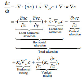 (5)
(5)where 


In addition, there are two components in the local total Adv: one due to the flux gradient 

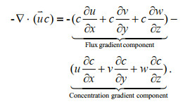 (6)
(6)According to the mass continuity, the sum of the former components, 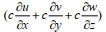
In the following analyses, the depth-averaged and volume-average variables are analysed. The square bracket denote the volume average within the cylinder. For example, [c] represent the depthaveraged and volume-average tracer concentrations in the cylinder.
2.4 Eddy detection and tracking methodThe eddy detection and tracking method used in this paper is from the method of Dong et al. (2011), which is based on the geometric characteristics of the flow field proposed by Nencioli et al. (2010). The eddy identification constraint condition defaults that the center of the eddy has the lowest velocity; the velocities on the east and west (north and south) sides of the eddy center have opposite numerical signs, the magnitude increases linearly with the distance from the center point; the rotation direction of the velocity vector must be consistent in the vicinity of the eddy center.
The boundary of the eddy is defined as the maximum closed stream function around the eddy center. The radius of the eddy is the average distance from each point on the eddy boundary to the eddy center.
After determining the selected eddy center, the eddy trajectory is determined by comparing the location of the eddy center in continuous time. In simple terms, this step searches for the next closest polarity eddy within a 15-km search radius of the eddy center that was detected in the previous step. If such an eddy can be found, it will be regarded as a successor of the previous eddy, and the eddy will not become a successor of other eddies; then, it will be followed up. If no qualified eddy is found at this time, the search radius will be increased to twice the previous radius the next time. If no eddy is found, the evaluation of the eddy will be terminated.
2.5 Definition of mixed layer depth and eddy kinematic propertiesThe mixed layer depth (MLD) in the upper ocean is an important physical parameter to describe the upper ocean. There are many standards for the definition of the MLD, and the MLD calculated according to different standards may be slightly different. The MLD criterion used in this paper refers to the method of de Boyer Montégut et al. (2004): near the surface temperature threshold at 10-m depth, the threshold is 0.2 ℃.
Considering the balance between the Coriolis force and pressure gradient force, the surface geostrophic velocity anomalies can be derived from the following formula:
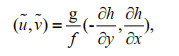 (7)
(7)in which ũ and ṽ are the zonal and meridional components of the geostrophic velocity anomalies, respectively. h is the sea level anomaly (SLA); g is the gravitational acceleration parameter; and f is the Coriolis parameter.
The eddy kinetic energy (EKE) is calculated from the geostrophic velocity anomaly component defined above using the relation:
 (8)
(8)PV is a dynamic conserved quantity describing the eddy rotation trend and is expressed as:
 (9)
(9)where ρ0 is the density parameter and 
The horizontal velocity divergence (Div) is defined as:
 (10)
(10)The nonlinearity of the eddy is measured by the following relation:
 (11)
(11)where the rotational speed U is defined to be the maximum mean geostrophic speed on the maximum closed PV contours, and 

The total deformation rate of the eddy, which means the degree to which the eddy shape deviates from a circular shape, is expressed as:
 (12)
(12)where 
The above definitions help to quantify the kinematic properties of eddies and are widely used to describe and study the various properties of eddies (Hwang et al., 2004; Chelton et al., 2011).
3 EDDY-INDUCED MASS TRANSPORT ESTIMATED BY A PASSIVE TRACERTo quantitatively estimate the eddy-induced mass transport, a typical AE (anticyclonic eddy) is chosen as our analysis object from the SCS simulation (cf. Section 2). The track of the eddy shows that this eddy first appeared in Southwest Taiwan, China, on November 23, 2012 and disappeared on March 2, 2013 (Fig. 2). During its lifetime of 100 days, the eddy travelled 689 km (Fig. 2), with an average radius reaching 68 km and a mean EKE of 462 cm2/s2, which is very strong. There was a weak steady background southwest flow along its track during its lifetime, with a mean depth-averaged (0–200 m) speed of < 2 cm/s. The zonal characteristic profiles of the eddy on the day of tracer initialization showed that the eddy had a symmetric bowl shape structure, with significant high temperatures, low salinity and low PV, corresponding to the typical characteristics of a strong warm eddy (Fig. 3a–c). The subsurface temperature (salinity) of the eddy center is 3 ℃ (0.2) higher (lower) than that outside the eddy. The MLD (solid black line in Fig. 3a & b) of the eddy center is approximately 30 m deeper than that outside the eddy, which coincides with the temperature and salinity (T-S) structure very well, suggesting that there is significant convergence and downwelling near the eddy center. The horizontal rotational velocity of the eddy is very strong, with its maximum reaching as high as 0.6 m/s (Fig. 3d). As a result, there is a significantly low PV region in the eddy core (Fig. 3c). The PV contours are not as smooth as those of T-S, suggesting that there are drastic temporal and spatial variabilities in PV and eddy deformation.

|
| Fig.2 Track of the eddy center during its lifetime (solid brown line) and the SLA (shading) on the day of tracer initialization from the model outputs The solid black dot is the eddy center where the eddy first appears, the white asterisk is the eddy center on the day of tracer initialization, and the solid green triangle is the eddy center on days 20, 40, 60, and 80 from the tracer initialization day. The grey contours are isobaths (unit: m). |

|
| Fig.3 Zonal profiles of temperature (a), salinity (b), PV (c), and meridional velocity (d) crossing the eddy center (along 21.4°N) on the day of tracer initialization The bold solid black line in (a) and (b) denotes the MLD. The dashed green line represents the edge of the eddy core. |
According to the PV distribution in each layer, the passive tracer is then initialized uniformly with a unit value (in arbitrary tracer units per volume, ATU/m3) in the eddy core on December 8, 2012 (Fig. 4a). Following Zhang et al. (2014), the core is defined as the area in the outermost closed contours of PV in each layer. In addition, the day of tracer initialization is set to 15 days after the first appearance of the eddy to avoid possible instability at the early stage of the eddy. Most of the tracer-tagged water falls between 21.9 and 23.5 kg/m3 in potential density, between 33.8 and 34.2 in salinity, and between 21 and 27 ℃ in temperature (Fig. 4b).

|
| Fig.4 A 3-D demonstration of the initial condition of tracer integration (a); initial distribution of tracer concentration (1010ATU) against temperature and salinity (b) The tracer was released on December 8, 2012, with a unit value (in arbitrary tracer units per value, ATU/m3) in the core of the eddy. The contours represent density (kg/m3), with a contour interval of 1 kg/m3. See the text for more details. |
As the eddy moves westward, the shape and volume of the eddy core continuously changes. Therefore, it is inappropriate for us to analyse the tracer variability in the changing eddy core. As an alternative, all tracer variability analyses in this study are performed in a fixed shape cylinder surrounding the moving eddy core (the cylinder in Fig. 4a). The cylinder axis is set vertically through the real-time surface eddy center, and the cylinder radius and depth are set as 85 km (1.2 times the average eddy radius, larger than 90% of the eddy radii at any time, and 100% that before day 65) and 200 m (97% of the tracers are found above this depth during the lifetime of the eddy), respectively. The eddy core is not completely wrapped in this cylinder at all times because the eddy radius becomes extra-large (~90 km) for 15 days before its termination.
The tracer is then released and traced forward in time under the control of the passive tracer module embedded in the SCS simulation of the ROMS model. The evolution of the tracer is described in detail in the following section.
3.1 The transport of tracerThe three-dimensional (3-D) distribution of the tracer concentration is presented as a function of days to clearly illustrate the process of mass transport by this eddy (Fig. 5). The tracer-tagged water initially trapped by the eddy core continuously leaked out of the eddy during the long-distance movement over 689 km. The red isosurface, which wraps the high concentration (>0.5 ATU/m3) tracer, shrank little by little, and disappeared at the time of termination. Meanwhile, the blue isosurface corresponding to the low concentration (>0.01 ATU/m3) gradually expanded to the periphery of the eddy. The distribution of the vertically integrated tracer (shading on the bottom plane in Fig. 5) also shows that a considerable amount of the tracer spread horizontally out of the eddy. The volume-averaged tracer concentration in the cylinder, [c], exhibited a significant decreasing trend, reaching as high as 1.0×10⁻³ ATU/(m3·d), which is equivalent to an average of 6‰ tracer spreading out of the cylinder per day (Fig. 6a). At the terminal time, approximately half of the (49%) tracers flowed out of the cylinder. This result confirms the strong mass transport capability of eddies, which has been proven by many previous studies (e.g., Early et al., 2011;
Dong et al., 2014; Zhang et al., 2014). However, the loss of tracers was also considerable, which should be considered when analysing the contribution of eddyinduced mass transport to large-scale circulation. A significant variation was superimposed on the decreasing trend of [c] (Fig. 6a). The temporal derivative of [c], 

|
| Fig.5 3-D spatial distribution of the tracer concentration on days 0 (a), 10 (b), 20 (c), 40 (d), 60 (e), and 85 (f) Four isosurfaces in different colours are plotted in the figure. Different colours correspond to different concentration values, in which red corresponds to 0.5 ATU/m3, yellow 0.3 ATU/m3, green 0.1 ATU/m3, and blue 0.01 ATU/m3. The shading on the bottom plane is the distribution of the vertically tracer volume-integration (ATU/m2), where the purple red circle represents the range of the moving cylinder (see Section 2.3 for details), the white point represents the position of the eddy center on the surface, and the black line represents the moving track. "Day" denotes the time, "Remain" denotes the percentage of the tracer remaining in the cylinder, and "Distance" displays the distance from the eddy center to its initial tracer position. The colorbar corresponds to the vertically tracer volume-integration (ATU/m2). |

|
| Fig.6 Time series (bold solid black line), trend (thin solid black line), and time derivative (dashed grey line) of the average tracer concentration in the cylinder during the lifetime of the eddy (a); time-depth distribution of the horizontally averaged tracer concentration (shading) and the centroid depth of the tracer-tagged water (solid black line) in the cylinder (b) The solid white line in (b) represents the horizontally averaged MLD in the cylinder. |
A warm eddy can produce significant convergence and dowelling (Hu et al., 2011; Dong et al., 2014; Sun et al., 2018). In this experiment, notable downwelling of tracer-tagged water was observed (Fig. 5). The centroid depth of the tracer-tagged water in the cylinder decreased 21 m (from 36 m to 57 m) during the eddy lifetime (Fig. 6b). Meanwhile, the MLD also shows a significant variation during the lifetime of eddy. The result indicates that the MLD got deepening in the first 50 days, reflecting the strengthening of the eddy during this period, which is conducive to the detraining of the tracer-tagged water. After that, the eddy entered into the decay period, leading to the shallowing of the MLD in the eddy. As a result, there were more detrained water remaining in the subsurface, which is a valid contribution of subduction. On the terminal day, 4.68×10¹⁰ m3 of tracer-tagged water detrained underneath the mixed layer, which accounted for 65% of the total water initially in the mixed layer of the eddy. The downward water flux induced by this warm eddy reached as high as 5×10⁴ m3/s, indicating the important contribution of the eddy to the vertical water exchange, which led to the corresponding eddy-induced subduction (Xu et al., 2016) and diabatic mixing (Bachman and Taylor, 2016), and consequently had a noticeable impact on water properties. However, the vertical circulation in the AE (warm eddy) was not found to represent uniform downwelling (Nardelli, 2013; Cotroneo et al., 2016; Pilo et al., 2018). A diploe pattern of convergence and divergence in the eddy core was also found in this experiment. The dynamics will be explored in more detail in a later section to show the structure of the vertical circulation of this eddy.
3.2 Impact on water characteristicsAs the eddy moves westward, the horizontal water exchange between the inside and outside of the eddy core significantly transforms the characteristics of the water in the eddy. Fifty days later, the temperature of the eddy decreases by as much as 3 ℃, while the salinity is almost unchanged (decreased by only 0.05), which is consistent with the low temperature and low salinity characteristics of the inflow water (Fig. 7c & d). The temperature difference between water in the eddy and that along the track of the eddy is very large (>5 ℃), but the difference in salinity between them is very small (< 0.2), and the salinity outside the eddy is even slightly fresher than that inside the eddy. Therefore, the variability in density (Fig. 7b) is mainly determined by temperature.

|
| Fig.7 Time-depth distribution of anomalies of horizontally averaged tracer concentration (a), density (b), temperature (c), and salinity (d) in the cylinder |
Meanwhile, eddy-induced vertical mass transport also significantly changes the T-S characteristics of subsurface water in the eddy. As shown in Fig. 7a, much surface water is subducted into the layer beneath the MLD of the eddy, and the subducted water then makes the subsurface water warmer, fresher, and lighter. Fifty days later, the subsurface temperature increases by 2 ℃ and salinity decreases by 0.2, resulting in a density decrease of 0.5 kg/m3 (Fig. 7b–d).
The tracer distributions against temperature and salinity (Figs. 8 & 9) further illustrate how the tracertagged water is transformed during the lifetime of the eddy. The core of the tracer has an initial density range roughly between 21.5 and 23.5 kg/m3, with temperature between 23 and 26 ℃ and salinity between 33.8 and 34.2 (Fig. 4b). As the tracer-tagged water moves with the eddy, its density increases gradually (Fig. 8). By day 40, the characteristics of the tracer are transformed into increased density (>23 kg/m3) and decreased temperature (< 22 ℃), which is mainly due to the merging of the horizontal influx of cold water. At the same time, a small portion of the water is transformed into much denser (25– 27 kg/m3) and colder (5–15 ℃) water, suggesting that a part of the surface water sank vertically into the subsurface and mixed with subsurface water to become colder and denser (Fig. 8), resulting in the local subsurface water becoming warmer and lighter (Fig. 7c & d). Unlike temperature, the variability in salinity is relatively weak both vertically and horizontally during this period (Figs. 7d & 8) due to the small salinity difference between the water inside and surrounding the eddy. By the terminal day, half of the tracer is still trapped in the cylinder, with its mean temperature decreasing by ~2.5 ℃ and density increasing by 1 kg/m3 (Fig. 9a), reflecting the significant effect of downwelling. Meanwhile, the other half of the tracer is spread outside of the cylinder (Fig. 9b). This result indicates that the temperature and density of the water that is still trapped in the cylinder are more concentrated, while that of the water that has leaked outside the cylinder are more dispersed (Fig. 9b).

|
| Fig.8 Distribution of tracer concentration (1010ATU) against temperature and salinity on days 20 (a), 40 (b), 60 (c), and 85 (d) over the entire region The contours represent density (kg/m3), with a contour interval of 1 kg/m3. |

|
| Fig.9 Same as Fig. 8 except that the region is inside (a) and outside (b) of the cylinder on the terminal day The contours represent density (kg/m3), with a contour interval of 1 kg/m3. |
As described in Section 3, eddy-induced tracer transport occurs in both the horizontal and vertical directions. On the one hand, a large amount of tracer disperses away from the eddy in the horizontal direction; on the other hand, considerable tracer sinks from the surface to the subsurface in the vertical direction. Meanwhile, according to the Eq.3, the two parts of transport are actually controlled by two ocean dynamic processes, advection and mixing. Therefore, it is of great significance to quantitatively study the effects of the different processes on tracer transport. However, due to the lack of observations, the role of these processes in eddy-induced mass transport has remained obscure.
In this section, by using the daily averaged results of all terms in Eq.3 from ROMS and the tracer budget method described in Section 2.3, a tracer budget in a cylinder moving with the eddy center is examined in detail. The temporal mean state, horizontal distribution, vertical structure, and temporal variability of the tracer budget are discussed.
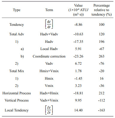
4.1 Mean state 4.1.1 Mean value and horizontal distributionThe spatial distribution and mean value of tracer budget terms in the cylinder are presented in Fig. 10 and Table 1. For the mean state, the temporal tendency term 

|
| Fig.10 Horizontal distribution of temporal mean depth-averaged (0–200 m) tracer budget terms over the cylinder, including Tendency (a), Total Adv (b), Total Mix (c), Horizontal Process (d), Hadv (e), Hmix (f), Vertical Process (g), Vadv (h), Vmix (i), local tendency (j), local total Adv (k), and coordinate correction (l) The black circle is the boundary of the cylinder, and the white contour indicates the zero value. The unit is ATU/(m3·s). A different color bar is used in (j), (k), and (l). |
|
As a major component, the distribution of Total Adv looks not fully axisymmetric, with a strong divergence center slightly southwest biased (Fig. 10b). Considering that the eddy propagation direction is southwestward, it seems that in the moving cylinder coordinates, the Total Adv tends to spread the tracer from the posterior of the eddy (relative to the propagation direction of the eddy, hereinafter the same), where the concentration increases. However, the situation in the Earth coordinate system is quite different. The local total Adv has a distinct dipole pattern, with a convergence zone in the anterior of the eddy and a divergence zone in the posterior of the eddy (Fig. 10k), which is in good agreement with the depth-averaged vertical velocity field of the upper layer (Fig. 11b). On the upper 100 m, the horizontal velocity field in the southeast (left side of the eddy, relative to the propagation direction, hereinafter the same) is much stronger than that in the northwest (right side of the eddy, Fig. 11a), which consequently leads to a significant convergence (downwelling) zone and a divergence (upwelling) zone in the anterior and posterior of the eddy respectively (Fig. 11b & c). In a recent study, an AE located in the Northwest Pacific was observed by using Argo float data (Dai et al., 2020). The geostrophic velocity at 200 db of this eddy was stronger in the south and weaker in the north, which is consistent with our results. A study by Cotroneo et al. (2016) provided a better observational evidence for the dipole pattern. In their study, an AE in the area between the Balearic Islands and the Algerian coast was observed in a deep glider cruise. The calculated vertical quasi-geostrophic velocity field presented a dipole pattern quite similar to our results, with relatively strong downwelling in the western part of the eddy and upwelling in the southeastern part, which lead to significant anomaly in chlorophyll concentration. Moreover, Pilo et al.
(2018) analysed 3 warm eddies in the East Australian Current region using a global eddy-resolving model. In their study, the temporal mean depth-averaged (0–2 000 m) vertical velocity for each eddy as they propagated along the tracks all showed significant dipole patterns similar to our result. They suggested that the dipole pattern was mainly induced by eddy distortion. However, there seems to be a simpler explanation. Many previous studies (Chelton et al., 2007, 2011; Early et al., 2011) suggested that a mesoscale eddy can be regarded as a nondispersive baroclinic Rossby wave; therefore, the dipole pattern seems to be well explained by the "β effect" 

|
| Fig.11 Horizontal distribution (upper row) of the temporal mean depth-averaged horizontal velocity (a), vertical velocity (b), and divergence (c) in the upper 100 m of the cylinder, and vertical section (lower row) of the temporal mean normal velocity (d), tangential velocity (e), and divergence (f) along the diagonal from northeast to southwest and through the eddy center (the solid black line in (a)) The quivers and blue lines superimposed in (d) and (e) are the tangential-vertical velocity vector and stream lines in the Earth coordinates and cylinder moving coordinates, respectively. |
According to the classical theory of the eddy pumping mechanism (Falkowski et al., 1991; McGillicuddy et al., 1998), a significant convergence (downwelling) zone symmetrically located around the eddy center is regarded as a symbolic feature of a warm eddy, which is indeed consistent with the observed symmetric distribution of temperature/ salinity/MLD in the composite analyses by many previous studies (e.g., Sun et al., 2018). In our study, a symmetric pattern of the tracer tendency also indicates that the water mass transport by eddies is isotropic. However, this result is only valid in the coordinates moving with the eddy. In the Earth coordinates, the divergence field of the eddy has a significant dipole pattern (Fig. 11c), with a strong convergence (divergence) in the anterior (posterior) direction, which is exactly the driving mechanism by which the eddy propagates westward. Note that the Total Adv (Fig. 10b) is one order of magnitude smaller than the local total Adv (Fig. 10k) due to the offset by the coordinate correction (Fig. 10l), which indicates that the dipole of convergence and divergence of the eddy in Earth coordinates is much stronger than the weak spreading pattern in the eddy moving coordinates. The dipole of convergence and divergence is bound to produce a corresponding strong downwelling zone and upwelling zone, which will certainly reflect the vertical structure of the eddy.
4.1.2 Vertical structureConsidering that the horizontal distribution of most tracer budget terms is nearly symmetrical with respect to the eddy propagation direction (31° west by south), the temporal mean tracer budget terms on the vertical section along the propagation direction and through the eddy center (the black solid line in Fig. 11a) are examined as follows, with particular attention to the vertical structure of the dipole of convergence and divergence (Fig. 12).

The tendency term (Fig. 12a) shows an axisymmetric spreading pattern consistent with its horizontal distribution (Fig. 10a). c in the eddy core decreases significantly, while it increases around the core and below the mixing layer, indicating that a large proportion of water subducts to the subsurface. The Total Adv and Total Mix in this section appear to have the same order of magnitude and partially counterbalance each other. Overall, however, the effect of Total Adv (65%) is still dominant and is 1.8 times larger than that of Total Mix (35%). As the main component of Total Mix, Vmix has an obvious feature: it is mainly confined in the mixed layer, and the effect under the mixed layer decreases sharply, illustrating the strong Vmix in the mixed layer. Meanwhile, the effect of Hmix is very weak, but it is not confined in the mixed layer and can reach a deeper depth of 150 m.
It is striking that the vertical structures of Hadv and Vadv show four-cell patterns, and there is a strong offset between them (Fig. 12e & h), which leads to their sum (the total Adv) being one order of magnitude smaller than the individual values (Fig. 12b). One reason is that according to the mass continuity, the sum of its flux components, 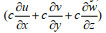

|
| Fig.13 Same as Fig. 12 except for the concentration gradient components in (a, c) and flux gradient components (b, d) of Hadv (a, b) and Vadv (c, d) |
Analogous to the horizontal distributions, the vertical distribution patterns of Total Adv and local total Adv (Fig. 12b & k) are also quite different. Since the Total Adv is a result of the eddy motion coordinates, it looks relatively weak, which indicates that the Total Adv has no strong impact on the leakage of the water mass from the eddy. However, from the viewpoint of the Earth coordinates, the local total Adv shows a significant dipole pattern of convergence and divergence in its vertical structure, which has been described in its horizontal distribution. On the left (right) side of the profile, the strong convergence and downwelling (divergence and upwelling) leads to a significant increase (decrease) in c penetrating the mixed layer to the subsurface, with its major influence depth reaching as deep as 100 m, which is in good agreement with the velocity field (Fig. 11). The quivers and streamlines in Fig. 11d show the tangential and vertical velocities on the profile in Earth coordinates. This indicates that in addition to the strong upwelling and downwelling, there is a net lateral flow in the eddy core, by which the subsurface upwelling water on the right side is transported to the convergence zone through the upper layer. As a consequence, the eddy core, which features the high c center, will be driven to shift towards the left. However, if we observe the velocity field in the cylinder moving coordinates (Fig. 11e), this surface lateral current disappears due to the coordinate correction and is replaced by an overturning cell. Through this overturning cell, the high c water first detrains from the surface layer of the left side of the eddy core to the subsurface by downwelling, then part of it merges into the upwelling zone of the right side and resurfaces and gradually spreads out by local divergence. A similar vertical structure can also be found in a group of anticyclonic eddies in the East Australian Current region simulated by Pilo et al. (2018). Of course, this velocity field on the profile represents only net transport; due to the fast swirl of the eddy, the real trajectory of the water mass is supposed to be spiral.
This result, however, is contrary to our knowledge that the AE core is uniformly downwelling (e.g., Paterson et al., 2007; Nemcek et al., 2008; Oliver and Holbrook, 2014). In particular, there seems to be a significant upwelling zone in the posterior of the eddy, which is likely correlated with eddy propagation.
4.2 Temporal variabilityFigure 14 shows the temporal variations in the tracer budget and its components averaged in the cylinder during the tracer experiment. This indicates (Fig. 14a) that the temporal variability of the tracer tendency is very significant, with its STD (3.3×10⁻⁸ ATU/ (m3·s)) 3.3 times its average (-1.0×10⁻⁸ ATU/(m3·s)), in which Hadv plays the most dominant role. The correlation coefficient (R) between Hadv and the tendency is 0.80, while all the other terms do not have a significant correlation with the tendency. As the second major factor, Vadv partially offsets the effect of Hadv. As a result, the correlation of the Total Adv with the tendency reaches as high as 0.99. The variability of the mixing terms is relatively mild, and the STD of Total Mix is only 1/5 of the Total Adv. The variability of Hmix is very weak, while the variability of Vmix is relatively large, barely comparable to that of Vadv.

|
| Fig.14 Temporal variation in the volume-averaged tracer budget (a) and the components of advection terms (b) in the cylinder during the experiment |
Further inspection of the individual components of the advection terms indicates that Hadv_c and Vadv_c are quite similar but with opposite signs, with their negative correlation reaching as high as 0.90 (Fig. 14b). The large degree cancellation between these two terms results in a reduced total advection that is one order of magnitude smaller. At the same time, due to the large cancellation between Hadv_flux (Vadv_flux) and Hadv_c (Vadv_c), Hadv (Vadv) is also reduced significantly. Please refer to Section 4.1.2 for the interpretation of the cancellations.
4.3 Correlation between eddy kinetic features and tracer budget termsPrevious studies (Chelton et al., 2011; Zhang et al., 2014) suggest that some eddy kinetic features are likely highly correlated with the eddy mass transport capability. Among others, the nonlinearity of eddies (N) is considered to be an important index of mass transport by eddies. As Chelton et al. (2011) pointed out that as long as N>1, there will be a parcel of trapped water mass within the eddy core that is transported with eddy propagation. Since the mean N of this eddy is 4.8 with its maximum reaching 8.5, the eddy in this study is supposed to have an excellent water mass trapping capability. Another feature that is considered to be possibly correlated with the mass transport of eddies is the deformation rate of eddies. According to its definition (Section 2.5), the physical meaning of γ is the degree in which the eddy shape deviates from the circular shape. Therefore, it is reasonable to assume that the larger γ is, the more irregular the eddy shape is, and the faster the tracer leaks. Moreover, the other features associated with the eddy intensity, such as EKE, U, radius, etc., are also possibly relevant to eddy mass transport.
Since the mass transport capability of the eddy can be quantified by the tendency term of the above tracer budget, i.e., the variability of the averaged tracer concentration in the cylinder, the correlations between the features and tracer budget terms of the eddy are then evaluated in detail as follows.
The period for all analyses in this section is set from the 15th day to the 65th day of the tracer experiment for 2 reasons. First, the volume of the initial tracer-tagged water is only 1/5 that of the cylinder, and there is a considerable blank area between the initial tracer region and the cylinder boundary (Fig. 4a). Therefore, it takes approximately 15 days for the initialized tracer to reach the boundary and start leaking from the cylinder, which results in the tendency term being nearly zero for the first 15 days (Figs. 6a & 14a). Second, the lifetime of a typical eddy is usually divided into three stages: youth, mature, and aged (Liu et al., 2012; Lin et al., 2015; Zhang et al., 2016). The first and last 20% of the lifetime is the "youth" stage and the "aged" stage, respectively. There are drastic variations in the state of the eddy during these two stages. Meanwhile, at the "mature" stage (the middle 60% of the lifetime), the status of the eddy is relatively stable (Lin et al., 2015). To avoid the impact of the different stages, the "mature" stage is chosen as the analysis period. Considering that the tracer experiment started on the 15th day when the eddy first appeared, the "mature" period was set from the 5th day to the 65th day of the experiment. As a result, the intersection of these two time periods was from the 15th day to the 65th day of the experiment (referred to as the "mature period" hereafter). In addition, the tendency is found to be low-frequency variability. Therefore, an 8-day low pass filter is applied to all the variables in the analyses to avoid the impact of the high frequency variations in the features. The power spectrum density analysis of the tendency term indicates that the remaining lowfrequency signal after filtering accounts for 85% of the total power.
Unexpectedly, the result indicates that N does not have a good correlation with the tendency. It seems that N does not directly impact the mass transport capability of the eddy. Meanwhile, neither U nor s show good correlations with the tendency. As Chelton et al. (2011) pointed out, N has a threshold; therefore, as long as it passes the threshold, i.e., N>1, the eddy could have a good mass transport capability.
However, further analysis indicates that one of the relevant parameters of N, the propagation acceleration of the eddy, 


|
Fig.15
Variability of tendency with a (a), Hadv with a (b), tendency with    |
γ is another feature that is considered possibly correlated with the mass transport of eddies. However, similar to the case of N, neither γ nor its two components, γ1 and γ2, have a significant correlation with tendency, but 


Similar analyses of many other features, such as the eddy radius, EKE, and PV, are also conducted; however, no high correlation with the tendency is found. Of course, it cannot be certain that eddy mass transport has nothing to do with these features because it is probably the result of the interaction of these features with different dynamics, which needs careful study in the future. For example, the EKE is highly positively correlated with the Vadv (R=0.74, Fig. 15f), while it is also negatively correlated with the Hadv (R=-0.53), and their interaction results in a poor correlation between EKE and the tendency.
However, the correlation of some temporal derivatives of eddy features (N and γ) with tendency is very significant, which suggests that the temporal instability of the eddy probably plays an important role in eddy mass transport. An eddy in drastic adjustment tends to leak extensive water mass from the eddy.
5 SUMMARY AND DISCUSSIONTo quantitatively investigate the water mass transport of oceanic mesoscale eddies, the mass transport induced by an AE in the SCS was evaluated by using a built-in simulated passive tracer of the ROMS model.
The results of the tracer experiment indicate that the eddy was robust and stable. It trapped and transported 51% of the initial tracer-tagged water in the eddy core to 689 km from its origin during its lifetime of 100 days, with a stable loss rate of approximately 6‰ per day. This result confirms the strong long-distance mass transport capability of mesoscale eddies, which has been proven by many studies (e.g., Early et al., 2011; Dong et al., 2014; Zhang et al., 2014). However, it also indicates that more than half of the water that was initially trapped by eddies leaked out of the eddy during eddy propagation, which suggests that it is necessary to quantitatively evaluate the loss quantitation when we analyse the contribution of eddy-induced mass transport to large-scale circulation.
During the propagation of the eddy, there was a dramatic horizontal water exchange between the inside and outside of the eddy core. Some tracertagged water that has flowed out of the cylinder may flow back into the eddy core. This result is consistent with the observations reported by Qiu et al. (2019). Meanwhile, the eddy-induced vertical mass transport was also very significant, and approximately 60% of the water initially in the mixed layer of the eddy was eventually detrained into the subsurface. As a result, the water in the mixed layer of the eddy became colder and denser, and the water in the subsurface became warmer and lighter.
To evaluate the effects of different dynamics on transport quantitatively, a tracer budget in a fixedvolume cylinder moving with the eddy center is examined in detail. The result indicates that advection is dominant, accounting for 120% of the tendency, while the effect of mixing is weak, explaining -20%. It is unexpected that the overall effect of the Total Mix on the tracer tendency is positive, which is mainly due to the contribution of Vmix. This suggests that mixing may help to conserve the water mass in eddies. This result is contrary to our common sense that mixing generally reduces the tracer concentration. The mechanism driving this result needs further study. The effect of the horizontal process is 2 times that of the vertical process, indicating that the horizontal process plays a controlling role in the mass transport of the eddy. Horizontal and vertical advection are found in opposite patterns and strongly offset each other.
The horizontal distribution and vertical structure of the local velocity field of the eddy all show distinct dipole patterns, which have significant convergence (downwelling) and divergence (upwelling) zones in the anterior and posterior of the eddy core, respectively. Due to the dipole, there is an overturning cell in the vertical direction, through which the surface water in the anterior of the eddy tends to detrain into the subsurface by downwelling and partially resurface from the posterior of the eddy by upwelling and gradually spreads out.
Because the vertical velocity in the mesoscale eddy is not easy to measure directly, less attention has been given to the vertical velocity in the eddy than to other aspects of eddy dynamics. An indirect method using the quasi-geostrophic Omega equation is applied in most studies of the vertical velocity of eddies (e.g., Martin and Richards, 2001; Hu et al., 2011; Nardelli, 2013), which, however, requires observations with high spatial and temporal resolution. In classic theories of the vertical velocity of an eddy, such as the eddy pumping mechanism (McGillicuddy et al., 1998), the vertical velocity in the eddy core and the corresponding downwelling (upwelling) zone should be centrosymmetric around the eddy center at all depths, which seems consistent with the observed symmetric distribution of temperature/salinity/MLD in the composite analyses by many previous studies (e.g., Zhang et al., 2014; Sun et al., 2018). By using satellite altimetry and Argo profiles, Sun et al. (2018) and others investigated eddies in the SCS. Their results indicated that the composite horizontal velocity field presents a fully symmetric structure around the normalized eddy-coordinate center at all depths. In our study, however, the vertical velocity within the eddy core presents a significant dipole pattern. Similar dipole patterns of vertical velocity were found in a recent model study of anticyclonic eddies in the East Australian Current region by Pilo et al. (2018). However, the dipole pattern was considered a result of eddy distortion in their study. A good observational evidence is also found in a study of Chelton et al. (2011), in which the Influence of mesoscale eddies on near-surface oceanic chlorophyll is analyzed using the satellite estimates. It can be seen in this study, there is a significant dipole pattern of the near-surface chlorophyll anomaly, with a negative (positive) anomaly in the anterior (posterior) of the eddy core, which obviously corresponds to the downwelling (upwelling). However, the dipole pattern of the chlorophyll anomaly is taken as a result of the interaction between the horizontal advection of eddies rotation and the meridional gradient of the chlorophyll distribution. In our opinion, if we consider the propagation of the eddy, it seems necessary to have such a constant dipole structure to drive the eddy to move westward and the occurrence of eddy distortion is not necessary. Therefore, it might be related to the driving mechanism for the westward propagation of the nondispersive baroclinic Rossby wave. As the dipole pattern is correlated with eddy propagation, eddies with different propagation speeds are likely to have different patterns, which requires a theoretical analysis in more detail. Moreover, since these results are only a model result of a single warm eddy, it is still uncertain whether these results can represent the situation of an eddy in the real ocean. Furthermore, the situation of a cold eddy seems quite different from that of a warm eddy (Nardelli, 2013). Therefore, it is necessary for us to perform further composite analyses on the vertical velocity of more different types of eddies.
The temporal variability in the tracer budget is found to be very significant, in which horizontal advection is dominant. The propagation acceleration and the temporal derivative of the deformation rate are highly correlated with the tendency term, suggesting the potential effect of the temporal instability of eddies on eddy mass transport. To date, most of the theoretical solutions related to mesoscale eddies (e.g., Jayne and Marotzke, 2002; Dong et al., 2014; Zhang et al., 2014; Yang et al., 2015) are constant or time-independent. This result reminds us that it is necessary to construct a time-dependent theoretical model of mesoscale eddies in which the temporal derivative terms are considered.
6 DATA AVAILABILITY STATEMENTThe datasets generated and analyzed during the current study are available from the corresponding author on reasonable request.
7 ACKNOWLEDGMENTSupercomputing resources were provided by High Performance Computing Center of Institute of Oceanology of Chinese Academy of Science. We also thank Dr. Ronghua ZHANG (Institute of Oceanology, Chinese Academy of Sciences) and Tangdong QU (University of California, Los Angeles) for their helpful advices. The authors would like also to thank reviewers for their comments and the developers of ROMS for open access to their code.
Electronic supplementary materialSupplementary material (Appendix) is available in the online version of this article at https://doi.org/10.1007/s00343-021-1069-y.
Bachman S D, Taylor J R. 2016. Numerical simulations of the equilibrium between eddy-induced restratification and vertical mixing. Journal of Physical Oceanography, 46(3): 919-935.
DOI:10.1175/JPO-D-15-0110.1 |
Barth A, Alvera-Azcarate A, Weisberg R H. 2008. A nested model study of the Loop Current generated variability and its impact on the West Florida Shelf. Journal of Geophysical Research: Oceans, 113(C5): C05009.
|
Chelton D B, Gaube P, Schlax M G, Early J J, Samelson R M. 2011. The influence of nonlinear mesoscale eddies on near-surface oceanic chlorophyll. Science, 334(6054): 328-332.
DOI:10.1126/science.1208897 |
Chelton D B, Schlax M G, Samelson R M, de Szoeke R A. 2007. Global observations of large oceanic eddies. Geophysical Research Letters, 34(15): L15606.
DOI:10.1029/2007GL030812 |
Cotroneo Y, Aulicino G, Ruiz S, Pascual A, Budillon G, Fusco G, Tintoré J. 2016. Glider and satellite high resolution monitoring of a mesoscale eddy in the algerian basin: effects on the mixed layer depth and biochemistry. Journal of Marine Systems, 162: 73-88.
DOI:10.1016/j.jmarsys.2015.12.004 |
Dai J, Wang H Z, Zhang W M, An Y Z, Zhang R. 2020. Observed spatiotemporal variation of three-dimensional structure and heat/salt transport of anticyclonic mesoscale eddy in Northwest Pacific. Journal of Oceanology and Limnology, 38(6): 1654-1675.
DOI:10.1007/s00343-019-9148-z |
de Boyer Montégut C, Madec G, Fischer A S, Lazar A, Iudicone D. 2004. Mixed layer depth over the global ocean: an examination of profile data and a profile-based climatology. Journal of Geophysical Research: Oceans, 109(C12): C12003.
DOI:10.1029/2004JC002378 |
Dong C M, Mcwilliams J C, Liu Y, Chen D K. 2014. Global heat and salt transports by eddy movement. Nature Communications, 5: 3294.
DOI:10.1038/ncomms4294 |
Dong C M, Nencioli F, Liu Y, McWilliams J C. 2011. An automated approach to detect oceanic eddies from satellite remotely sensed sea surface temperature data. IEEE Geoscience and Remote Sensing Letters, 8(6): 1055-1059.
DOI:10.1109/LGRS.2011.2155029 |
Early J J, Samelson R M, Chelton D B. 2011. The evolution and propagation of quasigeostrophic ocean eddies. Journal of Physical Oceanography, 41(8): 1535-1555.
DOI:10.1175/2011JPO4601.1 |
Falkowski P G, Ziemann D, Kolber Z, Bienfang P K. 1991. Role of eddy pumping in enhancing primary production in the ocean. Nature, 352(6330): 55-58.
DOI:10.1038/352055a0 |
Fukumori I, Lee T, Cheng B, Menemenlis D. 2004. The origin, pathway, and destination of Niño-3 water estimated by a simulated passive tracer and its adjoint. Journal of Physical Oceanography, 34(3): 582-604.
DOI:10.1175/2515.1 |
Gao S, Qu T D, Fukumori I. 2011. Effects of mixing on the subduction of South Pacific waters identified by a simulated passive tracer and its adjoint. Dynamics of Atmospheres and Oceans, 51(1-2): 45-54.
DOI:10.1016/j.dynatmoce.2010.10.002 |
Gao S, Qu T D, Hu D X. 2012. Origin and pathway of the Luzon undercurrent identified by a simulated adjoint tracer. Journal of Geophysical Research: Oceans, 117(C5): C05011.
|
Hu J Y, Gan J P, Sun Z Y, Zhu J, Dai M H. 2011. Observed three-dimensional structure of a cold eddy in the southwestern South China Sea. Journal of Geophysical Research: Oceans, 116(C5): C05016.
|
Hwang C, Chen S A. 2000. Circulations and eddies over the South China Sea derived from TOPEX/Poseidon altimetry. Journal of Geophysical Research: Oceans, 105(C10): 23943-23965.
DOI:10.1029/2000JC900092 |
Hwang C, Wu C R, Kao R. 2004. TOPEX/Poseidon observations of mesoscale eddies over the Subtropical Countercurrent: kinematic characteristics of an anticyclonic eddy and a cyclonic eddy. Journal of Geophysical Research: Oceans, 109(C8): C08013.
DOI:10.1029/2003JC002026 |
Jayne S R, Marotzke J. 2002. The oceanic eddy heat transport. Journal of Physical Oceanography, 32(12): 3328-3345.
DOI:10.1175/1520-0485(2002)032<3328:TOEHT>2.0.CO;2 |
Johnson W K, Miller L A, Sutherland N E, Wong C S. 2005. Iron transport by mesoscale Haida eddies in the Gulf of Alaska. Deep Sea Research Part II: Topical Studies in Oceanography, 52(7-8): 933-953.
DOI:10.1016/j.dsr2.2004.08.017 |
Large W G, McWilliams J C, Doney S C. 1994. Oceanic vertical mixing: a review and a model with a nonlocal boundary layer parameterization. Reviews of Geophysics, 32(4): 363-403.
DOI:10.1029/94RG01872 |
Lee M M, Marshall D P, Williams R G. 1997. On the eddy transfer of tracers: advective or diffusive. Journal of Marine Research, 55(3): 483-505.
DOI:10.1357/0022240973224346 |
Lee M M, Nurser A J G, Coward A C, de Cuevas B A. 2007. Eddy advective and diffusive transports of heat and salt in the Southern Ocean. Journal of Physical Oceanography, 37(5): 1376-1393.
DOI:10.1175/JPO3057.1 |
Lin X Y, Dong C M, Chen D K, Liu Y, Yang J S, Zou B, Guan Y P. 2015. Three-dimensional properties of mesoscale eddies in the South China Sea based on eddy-resolving model output. Deep Sea Research Part I: Oceanographic Research Papers, 99: 46-64.
DOI:10.1016/j.dsr.2015.01.007 |
Liu Y, Dong C M, Guan Y P, Chen D K, McWilliams J C, Nencioli F. 2012. Eddy analysis in the subtropical zonal band of the North Pacific Ocean. Deep Sea Research Part I: Oceanographic Research Papers, 68: 54-67.
DOI:10.1016/j.dsr.2012.06.001 |
Marshall J, Shuckburgh E, Jones H, Hill C. 2006. Estimates and implications of surface eddy diffusivity in the Southern Ocean derived from tracer transport. Journal of Physical Oceanography, 36(9): 1806-1821.
DOI:10.1175/JPO2949.1 |
Martin A P, Richards K J. 2001. Mechanisms for vertical nutrient transport within a North Atlantic mesoscale eddy. Deep Sea Research Part II: Topical Studies in Oceanography, 48(4-5): 757-773.
DOI:10.1016/S0967-0645(00)00096-5 |
McGillicuddy D J Jr, Robinson A R, Siegel D A, Jannasch H W, Johnson R, Dickey T D, McNeil J, Michaels A F, Knap A H. 1998. Influence of mesoscale eddies on new production in the Sargasso Sea. Nature, 394(6690): 263-266.
DOI:10.1038/28367 |
Moore A M, Arango H G, Di Lorenzo E, Cornuelle B D, Miller A J, Neilson D J. 2004. A comprehensive ocean prediction and analysis system based on the tangent linear and adjoint of a regional ocean model. Ocean Modelling, 7(1-2): 227-258.
DOI:10.1016/J.OCEMOD.2003.11.001 |
Moore A M, Arango H G, Lorenzo E D, Miller A J, Cornuelle B D. 2009. An adjoint sensitivity analysis of the southern California current circulation and ecosystem. Journal of Physical Oceanography, 39(3): 702-720.
DOI:10.1175/2008JPO3740.1 |
Nan F, He Z G, Zhou H, Wang D X. 2011. Three long-lived anticyclonic eddies in the northern South China Sea. Journal of Geophysical Research: Oceans, 116(C5): C05002.
DOI:10.1029/2010JC006790 |
Nardelli B B. 2013. Vortex waves and vertical motion in a mesoscale cyclonic eddy. Journal of Geophysical Research: Oceans, 118: 5609-5624.
DOI:10.1002/jgrc.20345 |
Nemcek N, Ianson D, Tortell P D. 2008. A high-resolution survey of DMS, CO2, and O2/Ar distributions in productive coastal waters. Global Biogeochemical Cycles, 22(2): GB2009.
|
Nencioli F, Dong C M, Dickey T, Washburn L, McWilliams J C. 2010. A vector geometry-based eddy detection algorithm and its application to a high-resolution numerical model product and high-frequency radar surface velocities in the southern California bight. Journal of Atmospheric and Oceanic Technology, 27(3): 564-579.
DOI:10.1175/2009JTECHO725.1 |
Oliver E C J, Holbrook N J. 2014. Extending our understanding of South Pacific gyre ''spin-up'': modeling the East Australian Current in a future climate. Journal of Geophysical Research: Oceans, 119(5): 2788-2805.
DOI:10.1002/2013JC009591 |
Paterson H L, Knott B, Waite A M. 2007. Microzooplankton community structure and grazing on phytoplankton, in an eddy pair in the Indian Ocean off Western Australia. Deep Sea Research Part II: Topical Studies in Oceanography, 54(8-10): 1076-1093.
DOI:10.1016/j.dsr2.2006.12.011 |
Pilo G S, Oke P R, Coleman R, Rykova T, Ridgway K. 2018. Patterns of vertical velocity induced by eddy distortion in an ocean model. Journal of Geophysical Research: Oceans, 123(3): 2274-2292.
DOI:10.1002/2017JC013298 |
Qiu C H, Mao H B, Liu H L, Xie Q, Yu J C, Su D Y, Ouyang J, Lian S M. 2019. Deformation of a warm eddy in the northern South China Sea. Journal of Geophysical Research: Oceans, 124(8): 5551-5564.
DOI:10.1029/2019JC015288 |
Qu T D, Gao S, Fukumori I, Fine R A, Lindstrom E J. 2008. Subduction of south pacific waters. Geophysical Research Letters, 35(2): L02610.
|
Qu T D, Gao S, Fukumori I. 2013. Formation of salinity maximum water and its contribution to the overturning circulation in the North Atlantic as revealed by a global general circulation model. Journal of Geophysical Research: Oceans, 118(4): 1982-1994.
DOI:10.1002/jgrc.20152 |
Shchepetkin A F, McWilliams J C. 2005. The regional oceanic modeling system (ROMS): a split-explicit, free-surface, topography-following-coordinate oceanic model. Ocean Modelling, 9(4): 347-404.
DOI:10.1016/j.ocemod.2004.08.002 |
Shou W W, Zong H B, Ding P X, Hou L J. 2018. A modelling approach to assess the effects of atmospheric nitrogen deposition on the marine ecosystem in the Bohai Sea, China. Estuarine, Coastal and Shelf Science, 208: 36-48.
DOI:10.1016/j.ecss.2018.04.025 |
Stevens D P. 1990. On open boundary conditions for three dimensional primitive equation ocean circulation models. Geophysical & Astrophysical Fluid Dynamics, 51(1-4): 103-133.
|
Sun W J, Dong C M, Tan W, Liu Y, He Y J, Wang J. 2018. Vertical structure anomalies of oceanic eddies and eddyinduced transports in the South China Sea. Remote Sensing, 10(5): 795.
DOI:10.3390/rs10050795 |
Tomczak M, Godfrey J S. 2003. Regional Oceanography: An Introduction. 2nd edn. Daya Publishing House, Delhi. 390p.
|
Visbeck M, Marshall J, Haine T, Spall M. 1997. Specification of eddy transfer coefficients in coarse-resolution ocean circulation models. Journal of Physical Oceanography, 27(3): 381-403.
DOI:10.1175/1520-0485(1997)027<0381:SOETCI>2.0.CO;2 |
Warner J C, Sherwood C R, Signell R P, Harris C K, Arango H G. 2008. Development of a three-dimensional, regional, coupled wave, current, and sediment-transport model. Computers & Geosciences, 34(10): 1284-1306.
|
Wilkin J L. 2006. The summertime heat budget and circulation of southeast New England shelf waters. Journal of Physical Oceanography, 36(11): 1997-2011.
DOI:10.1175/JPO2968.1 |
Wunsch C. 1999. Where do ocean eddy heat fluxes matter. Journal of Geophysical Research: Oceans, 104(C6): 13235-13249.
DOI:10.1029/1999JC900062 |
Xu G J, Dong C M, Liu Y, Gaube P, Yang J S. 2019. Chlorophyll rings around ocean eddies in the north pacific. Scientific Reports, 9(1): 2056.
DOI:10.1038/s41598-018-38457-8 |
Xu L X, Li P L, Xie S P, Liu Q Y, Liu C, Gao W D. 2016. Observing mesoscale eddy effects on mode-water subduction and transport in the North Pacific. Nature Communication, 7: 10505.
DOI:10.1038/ncomms10505 |
Yang G, Yu W D, Yuan Y L, Zhao X, Wang F, Chen G X, Liu L, Duan Y L. 2015. Characteristics, vertical structures, and heat/salt transports of mesoscale eddies in the southeastern tropical Indian Ocean. Journal of Geophysical Research: Oceans, 120(10): 6733-6750.
DOI:10.1002/2015JC011130 |
Yuan D L, Han W Q, Hu D X. 2006. Surface Kuroshio path in the Luzon Strait area derived from satellite remote sensing data. Journal of Geophysical Research: Oceans, 111(C11): C11007.
DOI:10.1029/2005JC003412 |
Zhang Z G, Wang W, Qiu B. 2014. Oceanic mass transport by mesoscale eddies. Science, 345(6194): 322-324.
DOI:10.1126/science.1252418 |
Zhang Z W, Tian J W, Qiu B, Zhao W, Chang P, Wu D X, Wan X Q. 2016. Observed 3D structure, generation, and dissipation of oceanic mesoscale eddies in the South China Sea. Scientific Reports, 6: 24349.
DOI:10.1038/srep24349 |