 2021, Vol. 39
Institute of Oceanology, Chinese Academy of Sciences
Article Information
- SUN Lina, ZHANG Jie, MENG Junmin
- Study on the propagation velocity of internal solitary waves in the Andaman Sea using Terra/Aqua-MODIS remote sensing images
- Journal of Oceanology and Limnology, 39(6): 2195-2208
- http://dx.doi.org/10.1007/s00343-020-0280-6
Article History
- Received Aug. 18, 2020
- accepted in principle Oct. 22, 2020
- accepted for publication Dec. 14, 2020


2 Technology Innovation Center for Ocean Telemetry, Ministry of Natural Resources, Qingdao 266061, China
Internal solitary waves (ISWs) with strong nonlinearity are frequently observed in stratified oceans. ISWs are widely distributed in the world's oceans, especially near rough topography regions in marginal seas and coastal zones. The Andaman Sea in the Indian Ocean has been a classic study region for ISWs for several decades. This region has a special submarine topographic structure and stable stratigraphy, and is considered one of the areas where ISWs are most commonly observed in the world (Jackson, 2007; Magalhaes and Da Silva, 2018).
Internal solitary waves were first observed in the Andaman Sea in 1965. Perry and Schimke observed ISWs with amplitudes of 40 m in the southern Andaman Sea, which was the first report of ISWs in the Andaman Sea (Perry and Schimke, 1965). Later, papers such as Osborne and Burch (1980) described ISWs that propagated eastwards, separated by distances of approximately 100 km in the southern Andaman Sea, with a maximum amplitude and horizontal velocity of 60 m and 2 m/s, respectively. However, in-situ ISW observations are very sparse in the Andaman Sea. The development of remote sensing technology provides an effective means for collecting ISW observational data. Vlasenko and Alpers (2005) and Shimizu and Nakayama (2017) investigated the generation of ISWs and secondary internal waves by using numerical simulations. Studies on the spatial and temporal distribution, generation, propagation, and dissipation mechanisms of ISWs in the Andaman Sea have been reported by using numerical simulations and remote sensing (Sun et al., 2019). Five potential generation locations of mode-1 long living ISWs were revealed in the Andaman Sea using remote sensing observations, and the waves from two potential generation sites between the Nicobar Islands appear to radiate waves in two opposite directions, toward the Andaman Sea and the southern Bay of Bengal (Raju et al., 2019). Unprecedented satellite images showing long-lived short-scale mode-2 internal waves have been documented in the Andaman Sea by nonhydrostatic and fully nonlinear numerical models (Magalhaes et al., 2020). ISWs in the Andaman Sea were remotely generated through energetic surface tide-topography interactions (Apel et al., 1985). Simultaneously, data from geostationary orbit satellites, such as GOCI (Kim et al., 2018), Himawari-8 (Lindsey et al., 2018), and the infrared radiometer VIIRS (Hu et al., 2019), have also been widely used to study ISWs. Satellite remote sensing images can be used not only to study the characteristics of ISWs, but also to invert the amplitude, wavelength, propagation velocity, and other parameters of ISWs (Yaroshchuk et al., 2016; Zhang et al., 2016; Sun et al., 2018).
As one of the most important parameters of ISWs, the propagation velocity is affected by various factors, such as the topography, pycnocline, and tidal currents, which can directly reflect the propagation characteristics of ISWs. Semidiurnal tides are the main driving force of ISWs on the continental shelf. Based on the distance between two or more packets of ISWs in a single image, the propagation velocity of ISWs can be calculated by assuming that the ISW group has the same period (12.42 h) as the semidiurnal tide (Porter and Thompson, 1999; Li et al., 2000; Zhao et al., 2004). However, this method ignores the propagation direction of ISWs, and ISWs will travel for several hundred kilometers during the long half-day tidal period. With the increasing enrichment of satellite remote sensing data, ISWs can be captured from two adjacent remote sensing images of the same location, and the propagation velocity of the ISWs can be calculated from the space displacement and time interval (Liu et al., 2014; Hong et al., 2015). This method has higher digital accuracy than the single-image method (Jackson et al., 2013). Although the existing satellite data are abundant, it is not easy to acquire and capture two sets of ISW images in the same scene acquired in a short time. This method is restricted by the remote sensing image resolution, satellite observation geometry, solar azimuth, altitude, and data acquisition and many other conditions play an important role (Jackson and Alpers, 2010). The time lag between the two sets of images used to calculate the propagation velocity should not be too short. There are many mixed pixels in remote sensing images with low spatial resolution due to the limitation of the resolution of the satellite sensor.
This paper presents results on the estimation of the propagation velocity of ISWs in the Andaman Sea tracked using 195 image pairs of MODIS imagery over the period from January 2014 to December 2018. A total of 562 ISWs were identified during the period and the results of the propagation velocity distribution of ISWs in the Andaman Sea are presented. This paper introduces satellite remote sensing imagery covering 5 years between January 2014 and December 2018, which is used to study the propagation velocity of ISWs in the Andaman Sea (Section 2). The method for calculating the propagation velocity of ISWs by remote sensing imagery and the method for theoretically calculating the propagation velocity of ISWs theoretically, are then presented (Section 3). Section 4 presents the analysis of the propagation velocity characteristics of ISWs in the Andaman Sea. Section 5 is the discussion. The last section presents the conclusion.
2 SATELLITE OBSERVATION DATAMODIS is one of the primary sensors onboard the Terra and Aqua satellites, which were launched in 1999 and 2002, respectively. MODIS is a passive moderate resolution imaging spectroradiometer with 490 detectors in 36 spectral bands ranging from 0.4 microns (visible light) to 14.4 microns (thermal infrared) with a maximum spatial resolution of 250 m and a scanning width of 2 330 km. The Terra and Aqua satellites pass through the equator at approximately 10꞉30 and 13꞉30 local time each day, respectively. The two satellites pass through the same position on the same day with an approximately 3-h time interval. In view of the unique orbital and band characteristics of Terra/Aqua MODIS, the advantages of obtaining MODIS images of the same location more than once a day are presented, and the propagation velocity of ISWs in the Andaman Sea is studied in this paper.
To estimate the propagation velocity of ISWs, we need a pair of images that capture the same packet at two different times. A total of 195 such image pairs with suitable combinations are selected in the Andaman Sea spanning 5 years between 2014 and 2018. The geo-locations of the leading wavefront of the ISW packet are traced by taking the central pixels of bright patches in the imagery. An ensemble of all such leading wavefronts is combined to produce a complete picture of ISWs over the Andaman Sea, as shown in Fig. 1a. The red curve represents the ISW wavefront from Terra-MODIS imagery, and the blue curve represents the ISW wavefront from Aqua-MODIS imagery. The ISWs are mainly distributed in the southern, central, and northern parts of the Andaman Sea. The propagation characteristics of ISWs are observed differently in the northern, central, and southern regions of the Andaman Sea.

|
| Fig.1 MODIS image of ISWs in the Andaman Sea a. the distribution map of ISWs in the Andaman Sea. The red curve represents the ISW wavefront from Terra-MODIS imagery, and the blue curve represents the ISW wavefront from Aqua-MODIS imagery; b. MODIS image acquired on 5 March 2014 at 07꞉05 UTC showing the ISWs around the northern Andaman Sea; c & d. MODIS image acquired on 13 March 2017 at 07꞉00 UTC showing the ISWs around the central and southern Andaman Sea, respectively. |
The propagation velocity of ISWs was determined by using two different satellites for the multitemporal image (MTI) method, and the leading crests in two different groups of ISWs were used for the tidal period image (TPI) method (Hong et al., 2015). The TPI method is mainly applicable to tidal ISWs, but has a slightly decreased accuracy. This result is because ISWs will change greatly under the influence of the external environment, such as the terrain and flow field, during long-distance propagation during the long tidal cycle. This paper studies the propagation velocity of ISWs in the Andaman Sea based on the MTI method using MODIS onboard National Aeronautics and Space Administration (NASA) Terra/ Aqua satellites.
The time interval between Terra and Aqua MODIS images was approximately three hours. During this interval, the ISWs could travel distances ranging from several kilometers to tens of kilometers. Therefore, the propagation velocity of ISWs is v=l/t, where l is the propagation distance of the ISW and t is the propagation time. Figure 2 shows the Terra and Aqua MODIS remote sensing images acquired on 13 March 2017, showing ISW signatures in the southern Andaman Sea. Only one of the wave packets was intercepted to clearly show the ISW bands in the remote sensing images. The coverage areas of the two images are displayed as the solid black box in Fig. 2a. Figure 2b & c shows the MODIS images acquired on 13 March 2017 at 04꞉00 and 07꞉00 UTC, respectively. To accurately obtain the propagation distance of ISWs acquired on Terra and Aqua MODIS images, the coverage areas used to calculate the propagation distance of ISWs are displayed as solid red boxes.

|
| Fig.2 ISW images acquired by Terra-MODIS (13 Mar. 2017 at 04꞉00 UTC) and Aqua-MODIS (13 Mar. 2017 at 07꞉00 UTC) in the southern Andaman Sea a. the coverage areas of the two images are displayed as the solid black box; b. MODIS images acquired on 13 March 2017 at 04꞉00 UTC; c. MODIS images acquired on 13 March 2017 at 07꞉00 UTC; solid red boxes in the b & c are the coverage areas used to calculate the propagation distance of ISWs. |
Figure 3 shows the intensity profiles across the transect lines in the area displayed as the solid red box in Fig. 2b & c. The blue curve represents the ISWs in the Terra-MODIS image, and the red curve represents the ISWs in the Aqua-MODIS image. The distances between the Terra and Aqua MODIS images were measured, as shown in Fig. 3, and the propagation velocity of ISWs was computed using a data acquisition interval of 3 h.

|
| Fig.3 Cross sections of the Terra-MODIS image (blue line) and the Aqua-MODIS image (red line) brightness (reflectance) The ISW propagation direction is from left to right. |
The famous nonlinear equation (Korteweg-de Vries (KdV) equation) describing the solitary wave characteristics was derived by Korteweg and de Vries (1895). Thus, the characteristics of a single soliton in the two-layer ocean model can be described by the KdV equation in dimensional form. The propagation velocity of ISWs can be determined theoretically by solving the KdV equation using water depth, ocean stratification, and background current information. The formula is as follows:
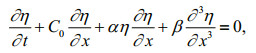 (1)
(1)where, t is time, η is the amplitude of ISWs, and C0 is the linear internal wave velocity, which is also a linear term. α and β are the first order nonlinear term coefficient and the dissipative term coefficient, respectively.
The shallow water term and dissipative term can be ignored if the viscous effect of seawater and the frictional effect of sea bottom are not considered. The solution for the above KdV equation is as follows:
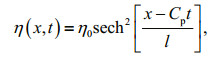 (2)
(2)where η0 is the amplitude of ISWs, Cp is the phase velocity of ISWs, and l is the half-wavelength of the ISWs.
For a two-layer mixed ocean system, the phase velocity Cp and half-wavelength l are:
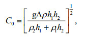 (3)
(3) (4)
(4)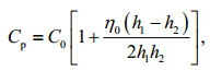 (5)
(5)where C0 is the linear velocity of ISWs, and h1, h2 is the thickness of the upper and lower layers, respectively. Δρ is the fluid density difference between two layers. ρ1, ρ2 is the density of the upper and lower layers, respectively. The theoretical speeds can be calculated from climatological stratification and bathymetry.
4 RESULT 4.1 Propagation velocity distribution of ISWsA total of 195 MODIS image pairs were acquired in the Andaman Sea in January 2014 and December 2018 from the NASA satellites Terra and Aqua. The morphology of 562 ISWs in the 195 image pairs was added to GIS software as shown in Fig. 4a. The crest lines of the different colors in Fig. 4a represent the ISWs detected by the different satellites. The red curves show the ISWs acquired by Terra, and the blue curves show the ISWs acquired by Aqua. The ISWs detected by Terra and Aqua on the same day were mainly distributed in the southern, central, and northern parts of the Andaman Sea, and most ISW pairs were detected in the southern Andaman Sea. The entire research area of the Andaman Sea was divided into 0.5°×0.5° cells, and the average propagation velocity of ISWs in each cell was calculated. The spatial distribution of the ISW propagation velocity is shown in Fig. 4b. The propagation velocity of ISWs in the deep sea of the central Andaman Sea was relatively fast, with a rate of approximately 3 m/s. In the southern and central parts of the Andaman Sea, the propagation velocity of ISWs decreases gradually in the process of transmission from west to east, and the velocities of ISWs in the shallow waters of the eastern coast are less than 1 m/s. The ISWs in the northern Andaman Sea are divided into two types. The first type of ISW was generated in the waters around the northern Andaman Sea islands and propagated eastward into the Andaman Sea. The ISWs of this type were significantly affected by topographic changes. Along the propagation direction of the ISWs, the water depth was shallow in the north and relatively deep in the south, which resulted in the propagation velocity of ISWs in the south being obviously higher than that in the north. Another type of ISW originates at the continental slope of the northern Andaman Sea and propagates southwest toward the Andaman Islands. The propagation velocity of ISWs was significantly reduced when it reached the sea area around the Andaman Sea islands.

|
| Fig.4 Distribution of the ISW crest line of the leading wave (a), propagation velocity (b), and theoretical propagation velocity (c) a. morphology of 562 ISWs in the 195 image pairs in January 2014 and December 2018 from the NASA satellites Terra and Aqua. The red curves show the ISWs acquired by Terra, and the blue curves show the ISWs acquired by Aqua; b. the spatial distribution of the ISW propagation velocity obtained by remote sensing; c. the diagrams of propagation velocity calculated by KdV equation. |
Figure 4c shows the diagrams of propagation velocity calculated by Eq.5. The propagation velocity of ISWs obtained by remote sensing corresponded with the results of the theoretical calculations. The propagation velocity of ISWs was almost consistent with the variation in water depth. The ISWs were distributed in water depths ranging from tens of meters to thousands of meters in this paper, and the propagation velocity of the ISWs increased gradually with the depth of water, as shown in Fig. 5, in which the propagation velocity was calculated by the 562 ISWs in the 195 image pairs in January 2014 and December 2018 from Terra and Aqua. The propagation velocity of ISWs was below 1 m/s when the water depth was less than 100 m, and the propagation velocity of the ISWs increased significantly with increasing water depth within the range of 200 m. When the water depth was below 500 m, the propagation speed of ISWs was less than 2 m/s. The propagation velocity of ISWs can reach more than 3 m/s when the depth is greater than 3 000 m. Since the upper layer depth does not vary greatly, the total water depth can show a strong correlation with ISW velocity. In general, the representative water depth is an essential factor.

|
| Fig.5 Relationship between the velocity of ISWs and the depth of water in the Andaman Sea The broken-dotted line is a fitting curve for propagation velocity and water depth. |
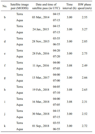
The propagation velocity of ISWs was affected by various factors; different ISWs may not have the same velocity at the same location, and the propagation velocity of ISWs at different times at the same location may not be different either. The propagation velocity of ISWs constantly changed throughout the life cycle. The propagation velocity of ISWs at the local scale was studied, where the central longitude and latitude were 95.3°E and 9.65°N, respectively. The water depth in the study area was approximately 2 500 m. Ten pairs of images were obtained that simultaneously detected ISWs spanning 5 years between 2014 and 2018 (Fig. 6b–k). The coverage areas of the study area are displayed as solid black boxes in Fig. 6a.

|
| Fig.6 Remote sensing images of ISWs matched by Terra and Aqua MODIS in the study area a. the coverage areas of the images are displayed as the solid black box; b. MODIS images acquired on 3 March 2014 at 04꞉15 and 07꞉15 UTC; c. MODIS images acquired on 24 January 2015 at 04꞉15 and 07꞉15 UTC; d. MODIS images acquired on 28 November 2015 at 03꞉55 and 06꞉55 UTC; e. MODIS images acquired on 28 February 2016 at 04꞉20 and 07꞉20 UTC; f. MODIS images acquired on 11 April 2016 at 04꞉00 and 07꞉05 UTC; g. MODIS images acquired on 13 March 2017 at 04꞉00 and 07꞉00 UTC; h. MODIS images acquired on 19 February 2018 at 04꞉05 and 07꞉10 UTC; i. MODIS images acquired on 16 March 2018 at 04꞉00 and 07꞉05 UTC; j. MODIS images acquired on 30 March 2018 at 04꞉15 and 07꞉15 UTC; k. MODIS images acquired on 1 September 2018 at 03꞉55 and 06꞉55 UTC. |
The propagation velocity of ISWs in the study area can be obtained by using the above 10 pairs of remote sensing images, as shown in Table 1. Due to the depth of water in this region, the propagation velocity of ISWs was relatively fast, ranging from 2.31 to 3.27 m/s. The propagation velocity of ISWs varies greatly in areas with the same water depth. The maximum propagation velocity of 3.27 m/s was estimated on 24 January 2015, and the minimum propagation velocity of the ISWs of 2.31 m/s was obtained on 16 March 2018. Figure 7 shows the average monthly propagation velocity of the ISWs in the study area. The propagation velocity of ISWs varies at the same water depths and shows certain seasonal variations, in which the maximum propagation velocity of ISWs occurs in January.
|

|
| Fig.7 Average monthly velocity of ISWs in a small region of the central Andaman Sea The black curve represents the propagation velocity of ISW obtained by remote sensing image, the red curve represents the propagation velocity of ISW calculated by KdV equation. |
The propagation velocity of ISWs was influenced not only by topographic depth but also by the stratified structure of the ocean. The change in season causes a change in sea temperature, followed by a change in the depth of the ocean mixing layer, which affects the propagation velocity of ISWs. Figure 8 shows the seasonal variation curves of temperature, salinity, density, and buoyancy frequency in the study area. Different colors represent the temperature, salinity, density, and buoyancy frequency curves of different months. The propagation velocity of ISWs in the deep mixing layer in January was higher than that in the shallow mixing layer in April. This result shows that monthly stratification plays a vital role in controlling the ISWs in the Andaman Sea.

|
| Fig.8 Vertical temperature, salinity, density, and buoyancy frequency profiles for the different seasons |
There were two types of ISWs in the northern Andaman Sea. The first type of ISW was generated in the northern Andaman Sea islands and propagated eastward into the Andaman Sea, eventually dissipating on the eastern continental shelf of the Andaman Sea. Another type of ISW originates at the continental slope of the northern Andaman Sea and propagates southwest toward the Andaman Islands, eventually dissipating on the continental shelf near the northern Andaman Islands. Figure 9a shows a MODIS image acquired on 19 March 2014 containing ISWs with two propagation directions. Three groups of ISW packets that were seaward propagate toward the northern Andaman Sea. Three groups of ISW packets propagating southwest toward the Andaman Islands were visible in the sea. Twenty pairs of remote sensing images of ISW in the northern Andaman Sea were used to calculate the propagation velocity of ISW in both directions, as shown in Fig. 9b. The red dot indicates the propagation velocity of ISWs traveling southwest, and the blue box indicates the propagation velocity of ISWs traveling southeast in the northern Andaman Sea. The propagating velocity of the ISW in the west direction is significantly higher than that in the east direction where the water depth is less than 500 m. The propagation velocity of the ISW is similar at water depths of 1 000–2 500 m, but overall, the velocity of the ISW propagating westward was higher than that of the ISW propagating eastward at the same depth in the northern Andaman Sea.

|
| Fig.9 The MODIS image of the northern Andaman Sea acquired on 19 March 2014 (a); the velocity of ISWs in the northern Andaman Sea (b) a. the blue figure represents the ISW packets that were seaward propagate toward the northern Andaman Sea; the red figure represents the ISW packets propagating southwest toward the Andaman Islands; b. the red dots represent the velocity of the ISWs propagating from the east to the North Andaman Islands, and the blue boxes show the velocity of the ISWs propagating from the west to the Andaman Sea. |
The propagation velocity of ISWs increased rapidly at depths below 1 000 m, while the propagation velocity did not increase significantly at depths between 1 000 m and 2 500 m. The propagation velocity was mainly concentrated in the range of 2.0–2.5 m/s. The velocity of the ISWs propagating westward was obviously larger than that of the ISWs propagating eastward at the same depth in the northern Andaman Sea. We believe this difference was probably caused by the change in topography. Figure 10 displays the change in water depth along the direction of the principal axis of ISW propagation. The blue curves show the ISWs propagating southeast toward the continental shelf, and the red curves show the ISWs propagating southwest toward Andaman Island. ISWs propagating southwestward were generated at the slope break of the northern Andaman Sea and then propagated to the deep sea in the southeast direction; the depth did not change significantly along the crestline of ISWs. ISWs propagating eastward were generated in the North Andaman Islands and propagated southeast into the Andaman Sea, and the topography along the crestline of ISWs changed significantly. The depth in the northern sea was shallow, and the water depth in the southern sea was relatively deep. This difference leads to a large difference in the propagation velocity of the same ISWs, which was fast in the south and slow in the north, thus affecting the overall propagation velocity of the ISWs.

|
| Fig.10 Topography profiles along the propagation direction of ISWs in the northern Andaman Sea a. distribution and propagation direction of internal solitary waves in the northern Andaman Sea, the blue curves show the ISWs propagating southeast toward the continental shelf; the red curves show the ISWs propagating southwest toward Andaman Island. The black arrow indicates the direction of internal solitary wave propagation; b. water depth curve of internal solitary waves propagating in two directions, the blue curve shows the depth profile of ISWs propagating eastward; the red curve shows the depth profile of ISWs propagating westward. |
The ISWs in the southern Andaman Sea were mainly generated in the ridge near the Gretel Strait and propagated eastward into the Andaman Sea. The black rectangle shown in Fig. 11a is the study area. Along the propagation direction of ISWs, the water depth gradually decreases, and the propagation velocity of ISWs gradually increases with increasing water depth. When the water depth was more than 1 500 m, the propagation velocity of ISWs did not increase with increasing water depth but tended to remain stable and even decreased. This finding was mainly due to the ISWs produced in the gray ridge near the strait, which spread eastward into the Andaman Sea. ISWs first spread into the sea area that was more than 2 000-m deep; the ISWs were still in the process of growth in this phase, and the growth process of ISWs strengthened. However, the propagation velocity was not the largest in the deep-sea portion of the study area. As the ISWs continue to travel eastward, their strength gradually increases, and their propagation velocity reaches a maximum of 2.8 m/s at depths of 1 200–1 500 m. ISWs continue to travel to the eastern coast, their velocity gradually decreases with decreasing water depth, and the minimum value is approximately 0.54 m/s.

|
| Fig.11 Variation in propagation velocity and water depth of ISWs in the southern Andaman Sea a. distribution of internal solitary waves in the southern Andaman Sea, the black rectangle shows the extent of the study area in the southern Andaman Sea. b. the variation of the propagation velocity of internal solitary wave with water depth, different shapes of scattered points represent the propagation velocity of internal solitary waves in different months. |
The propagation velocity of the ISWs was calculated based on the Terra/Aqua MODIS remote sensing images covering the southern Andaman Sea from January 2014 to December 2018. The average propagation velocity of ISWs was calculated by month and water depth (Fig. 12). The different colored columns represent the propagation velocity of the ISWs in different months. The propagation velocity of ISWs in different months varied greatly with the change in water depth, and the propagation velocity of ISWs in shallow water areas varied greatly. For water depths below 100 m, the velocity of ISWs can reach 1.9 m/s in August, while the average velocity in May is only 0.54 m/s. At water depths of 1 300–1 700 m, the maximum velocity of ISWs was 2.8 m/s in May. In general, the average velocity of ISWs increases with increasing water depth, as shown in the yellow column in Fig. 12.

|
| Fig.12 The propagation velocity of the ISWs in the southern Andaman Sea varies with the water depth from 1 to 12 months The yellow column represents the monthly mean propagation velocity of ISWs. |
In this paper, the propagation velocity of ISWs in the Andaman Sea was demonstrated in detail, rather than just individual cases in a typical region. Although the existing satellite data are abundant, it is not easy to acquire and capture two sets of ISW images in the same scene. This is restricted by the remote sensing image resolution, satellite observation geometry, solar azimuth, altitude, and data acquisition and many other conditions play an important role. There are many mixed pixels in remote sensing images with low spatial resolution due to the limitation of the resolution of the satellite sensor. The time lag between the two sets of images used to calculate the propagation velocity should not be too long or too short. If the time is too long, internal solitary waves will be affected by the external environment such as topography during their propagation and the propagation direction will also change, so that the propagation velocity calculated is not accurate. If the time lag is too short, the ISWs travel a distance of only a few pixels, this will cause large errors to the calculation of propagation velocity. Terra and Aqua are two satellites that cooperate with each other in time and space, and two images were effectively obtained at the same point on the same day, with a time interval of approximately 3 h. The remote sensing images used in this paper cover the Andaman Sea every month and the typical occurrence area of ISWs, which allowed the propagation velocity of ISWs to be detected.
However, only 195 pairs of MODIS image were matched in the Andaman Sea in January 2014 and December 2018. Thus it can be seen the data acquisition is valuable. Scanning width of the data used in this paper is 2 330 km, which can obtain a complete wave crest line with a length of hundreds of kilometers. The spatial resolution of the data used is 250 m, the position error of the extracted internal solitary wave in the remote sensing image is about 1 pixels. This distance is miniscule compared to the long distance of the internal solitary wave in three hours. Therefore, the position error of the extracted internal solitary wave has little influence on the calculation results of propagation velocity.
The propagation velocity of ISWs has a certain regional character and affected by various factors, such as the topography, pycnocline, and tidal currents. The results in this paper were consistent with existing reports that water depth was one of the important factors affecting the propagation of ISWs. Overall, the propagation velocity of ISWs increases with increasing depth. It was found that the propagation velocity of ISWs differed throughout the same range. A 0.7°×0.7° area in the central Andaman Sea was taken as the study area, where the water depth was approximately 2 500 m. The research shows that the propagation velocity of ISWs within this range exhibited great differences. In the season with a deep mixing layer, the propagation velocity of ISWs within this range was relatively large. This result indicates that the depth of the pycnocline was another important factor affecting the propagation velocity of the ISWs. Under the influence of the external environment, the propagation velocity of the ISWs varies seasonally, where the propagation velocity of ISWs in shallow water areas exhibits significant seasonal variation mainly because the shallow water area is greatly affected by the light and the external environment, and the seasonal thermocline changes significantly, while the thermocline in the deep water area is relatively stable.
For the ISWs in the northern Andaman Sea, there are two types of ISWs. The first type of ISW was generated in the northern Andaman Sea islands and propagated eastward into the Andaman Sea, eventually dissipating on the eastern continental shelf of the Andaman Sea. Another type of ISW originates at the continental slope of the northern Andaman Sea and propagates southwest toward the Andaman Islands, eventually dissipating on the continental shelf near the Northern Andaman Island. The velocity of the ISWs propagating in the west direction was obviously higher than that of the ISWs propagating in the east direction at the same water depth, which was mainly affected by the change in topography. This difference was mainly because the ISWs propagating to the west were located in the deep sea along the direction of the wave crest line of the ISWs, where there were limited changes in water depth. For the ISWs propagating eastward, along the direction of the wave crest line of the ISWs, the shallow sea continental shelf area was located to the north, and the deep-water area was located to the south. This condition results in an ISW traveling at different speeds from north to south, and then the whole propagation velocity of the ISWs is affected.
The propagation velocity of ISWs plays a very important role in the study of their propagation characteristics and prediction, and is also one of the key parameters in the numerical simulation of ISWs. Therefore, the propagation velocity of ISWs has important academic research value. The results of the study on the propagation velocity of ISWs will provide a valuable scientific basis for the study of the propagation and prediction of ISWs in the Andaman Sea. Unfortunately, due to the limitation of satellite remote sensing data and the propagation characteristics of the ISWs themselves, the propagation velocity of the ISWs on the continental shelf of the shallow sea could not be detected. The detection of the velocity in these areas requires satellite remote sensing data with higher resolution or results obtained by numerical inversion.
6 CONCLUSIONThe Andaman Sea has been a classic study region for ISWs because of its special geographical location and climate. As one of the important parameters of ISWs, propagation velocity has important research significance. The propagation velocity of the ISWs was calculated based on 195 MODIS image pairs acquired in the Andaman Sea in January 2014 and December 2018 from the NASA satellites Terra and Aqua. A total of 562 ISWs were identified during the period, and the results of the propagation velocity distribution of ISWs in the Andaman Sea were presented. The velocity distribution of ISWs in the Andaman Sea was plotted using a 0.5°×0.5° grid, and the distribution of the propagation velocity of ISWs in the Andaman Sea was obtained. The propagation velocity distribution of ISWs in the Andaman Sea was consistent with the distribution of water depth. The propagation velocity of ISWs in the deep area in the central and western regions was relatively high. The maximum propagation velocity of 3.27 m/s was estimated on the western side of the Nicobar Islands, and the minimum speed was 0.54 m/s in the shallow water region of the southeastern Andaman Sea. ISW propagation characteristics were observed to differ in the northern, central, and southern regions of the Andaman Sea. The propagation velocity in this paper focuses on the three main occurrence regions of ISWs in the Andaman Sea.
In the northern Andaman Sea, the velocity of the ISWs propagating westward was greater than that of the ISWs propagating eastward at the same water depth in the northern Andaman Sea. In the central part of the Andaman Sea, the propagation velocity of ISWs was studied in a 0.7°×0.7° grid area with a water depth of 2 500 m. The propagation velocity of ISWs in the deep mixing layer in winter was higher than that in the shallow mixing layer in summer. In the southern Andaman Sea, the monthly variations in ISW propagation velocity were analyzed. The velocity of ISWs differed greatly in shallow water and was not significantly different in deep water. In general, the average velocity of ISWs increases with increasing water depth. The results indicate that water depth and monthly stratification play a vital role in controlling the propagation velocity of ISWs in the Andaman Sea.
7 DATA AVAILABILITY STATEMENTSequence data that support the findings of this study have been deposited in the NASA Worldview application (https://worldview.earthdata.nasa.gov).
8 ACKNOWLEDGMENTWe thank the NASA MODIS Rapid Response System website announced that swath images.
Apel J R, Thomson D R, Tilley D G, Van Dyke P. 1985. Hydrodynamics and radar signatures of internal solitons in the Andaman Sea. John Hopkins APL Technical Digest, 6(4): 3330-3337.
|
Hong D B, Yang C S, Ouchi K. 2015. Estimation of internal wave velocity in the shallow South China Sea using single and multiple satellite images. Remote Sensing Letters, 6(6): 448-457.
DOI:10.1080/2150704X.2015.1034884 |
Hu S S, Ma S, Yan W, Hindley N P, Zhao X B. 2019. Measuring internal solitary wave parameters based on VIIRS/DNB data. International Journal of Remote Sensing, 40(20): 7805-7816.
DOI:10.1080/01431161.2019.1608389 |
Jackson C R, Alpers W. 2010. The role of the critical angle in brightness reversals on sunglint images of the sea surface. Journal of Geophysical Research: Oceans, 115(C9): C09019.
DOI:10.1029/2009JC006037 |
Jackson C R, da Silva J C B, Jeans G, Alpers W, Caruso M J. 2013. Nonlinear internal waves in synthetic aperture radar imagery. Oceanography, 26(2): 68-79.
DOI:10.5670/oceanog.2013.32 |
Jackson C. 2007. Internal wave detection using the Moderate Resolution Imaging Spectroradiometer (MODIS). Journal of Geophysical Research: Oceans, 112(C11): C11012, https://agupubs.onlinelibrary.wiley.com/doi/full/10.1029/2007JC004220.
|
Kim H, Son Y B, Jo Y H. 2018. Hourly observed internal waves by geostationary ocean color imagery in the East/ Japan Sea. Journal of Atmospheric and Oceanic Technology, 35(3): 609-617.
DOI:10.1175/JTECH-D-17-0049.1 |
Korteweg D J, de Vries G. 1895. On the change of form of long waves advancing in a rectangular canal, and on a new type of long stationary waves. The London, Edinburgh, and Dublin Philosophical Magazine and Journal of Science, 39(240): 422-443.
DOI:10.1080/14786449508620739 |
Li X, Clemente-Colon P, Friedman K S. 2000. Estimating oceanic mixed-layer depth from internal wave evolution observed from Radarsat-1 SAR. Johns Hopkins APL Technical Digest, 21(1): 130-135.
|
Lindsey D T, Nam S H, Miller S D. 2018. Tracking oceanic nonlinear internal waves in the Indonesian seas from geostationary orbit. Remote Sensing of Environment, 208: 202-209.
DOI:10.1016/j.rse.2018.02.018 |
Liu B Q, Yang H, Ding X W, Li X F. 2014. Tracking the internal waves in the South China Sea with environmental satellite sun glint images. Remote Sensing Letters, 5(7): 609-618.
DOI:10.1080/2150704X.2014.949365 |
Magalhaes J M, da Silva J C B, Buijsman M C. 2020. Long lived second mode internal solitary waves in the Andaman Sea. Scientific Reports, 10(1): 10234.
DOI:10.1038/s41598-020-66335-9 |
Magalhaes J M, da Silva J C B. 2018. Internal solitary waves in the Andaman Sea: new insights from SAR imagery. Remote Sensing, 10(6): 861.
DOI:10.3390/rs10060861 |
Osborne A R, Burch T L. 1980. Internal solitons in the Andaman Sea. Science, 208(4443): 451-460.
DOI:10.1126/science.208.4443.451 |
Perry R B, Schimke G. 1965. Large-amplitude internal waves observed off the northwest coast of Sumatra. Journal of Geophysical Research, 70(10): 2319-2324.
DOI:10.1029/JZ070i010p02319 |
Porter D L, Thompson D R. 1999. Continental shelf parameters inferred from SAR internal wave observations. Journal of Atmospheric and Oceanic Technology, 16(4): 475-487.
DOI:10.1175/1520-0426(1999)016<0475:CSPIFS>2.0.CO;2 |
Raju N J, Dash M K, Dey S P, Bhaskaran P K. 2019. Potential generation sites of internal solitary waves and their propagation characteristics in the Andaman Sea-a study based on MODIS true-colour and SAR observations. Environmental Monitoring and Assessment, 191(3): 809.
DOI:10.1007/s10661-019-7705-8 |
Shimizu K, Nakayama K. 2017. Effects of topography and Earth's rotation on the oblique interaction of internal solitary-like waves in the Andaman Sea. Journal of Geophysical Research: Oceans, 122(9): 7449-7465.
DOI:10.1002/2017JC012888 |
Sun L N, Zhang J, Meng J M. 2018. On propagation velocity of internal solitary waves in the northern South China Sea with remote sensing and in-situ observations data. Oceanologia et Limnologia Sinica, 49(3): 471-480.
(in Chinese with English abstract) DOI:10.11693/hyhz20171000259 |
Sun L N, Zhang J, Meng J M. 2019. A study of the spatial-temporal distribution and propagation characteristics of internal waves in the Andaman Sea using MODIS. Acta Oceanologica Sinica, 38(7): 121-128.
DOI:10.1007/s13131-019-1449-8 |
Vlasenko V, Alpers W. 2005. Generation of secondary internal waves by the interaction of an internal solitary wave with an underwater bank. Journal of Geophysical Research: Oceans, 110(C2): C02019.
DOI:10.1029/2004JC002467 |
Yaroshchuk I O, Leont'ev A P, Kosheleva A V, Pivovarov A A, Samchenko A N, Stepanov D V, Shvyryov A N. 2016. On intense internal waves in the coastal zone of the Peter the Great Bay (the Sea of Japan). Russian Meteorology and Hydrology, 41(9): 629-634.
DOI:10.3103/S1068373916090053 |
Zhang X D, Wang J, Sun L N, Meng J M. 2016. Study on the amplitude inversion of internal waves at Wenchang area of the South China Sea. Acta Oceanologica Sinica, 35(7): 14-19.
DOI:10.1007/s13131-016-0902-1 |
Zhao Z X, Klemas V, Zheng Q A, Li X F, Yan X H. 2004. Estimating parameters of a two-layer stratified ocean from polarity conversion of internal solitary waves observed in satellite SAR images. Remote Sensing of Environment, 92(2): 276-287.
DOI:10.1016/j.rse.2004.05.014 |