 2021, Vol. 39
Institute of Oceanology, Chinese Academy of Sciences
Article Information
- SHI Xingyu, WANG Zhenyan, HUANG Haijun
- Physical oceanography of the Caroline M4 seamount in the tropical Western Pacific Ocean in summer 2017
- Journal of Oceanology and Limnology, 39(5): 1634-1650
- http://dx.doi.org/10.1007/s00343-021-0359-8
Article History
- Received Sep. 21, 2020
- accepted in principle Nov. 16, 2020
- accepted for publication Jan. 21, 2021


2 Laboratory for Marine Mineral Resources, Pilot National Laboratory for Marine Science and Technology (Qingdao), Qingdao 266237, China;
3 University of Chinese Academy of Sciences, Beijing 100049, China;
4 Center for Ocean Mega-Science, Chinese Academy of Sciences, Qingdao 266071, China
Seamount is an underwater elevation rising generally more than 1 000 m and of limited extent across the summit (United States Board on Geographic Names, 1981; Rogers, 1994). As an obstacle to ocean currents, seamounts alter the ocean conditions locally and even globally (Lavelle and Mohn, 2010). Physical processes related to seamounts are thought to affect the local biota in a variety of ways, and make great contribution to the marine ecosystem (Clark et al., 2010; Rowden et al., 2010). Although many mechanisms have been questioned, there is no doubt that physical oceanography in seamounts plays a significant role in the sedimentation of particulate matter and the distribution of organisms (Genin, 2004; Shank, 2010).
Prevailing current will always deform when encountering a seamount. A Taylor cap may be induced when a steady flow pass over a seamount (Hogg, 1973), and it is marked by uplifted isotherms and will retain particulate matters, nutrients, and larvae transported by the advection or from the deep water, then attract organisms to gather together and form the unique populations of seamounts (Roden and Taft, 1985; Genin, 2004; Zhang and Xu, 2013). Periodic flows will also affect the seamount. The tidal rectification may be formed at the top of the seamount when the tidal currents flow through (White et al., 2007). This results in the generation of a cold and dense dome over the seamount, similar to the uplifted isotherms formed by a Taylor cap. It can also help to sustain biological and biologically important properties over the summit. In addition, as a muddler in the ocean, seamount can convert the tide energy into internal tides, induce circulation, and cause turbulent mixing near the seamount. Strong vertical mixing can increase the suspended particulate matters in the water column, provide well conditions for corals, sponges and other suspension feeders (Genin et al., 1986). Therefore, physical observations have also been made in many sedimentological and biological investigations of seamounts to assist the analysis of deposition process and biological distribution (Read and Pollard, 2017; Vianello et al., 2020).
The tropical Western Pacific Ocean is a typically oligotrophic water with relatively low productivity. In addition, the tropical Western Pacific Ocean is one of the most concentrated areas of seamounts. The ocean circulation in this area is complex and changeable, and it consists of several equatorial currents and the western boundary currents (WBCs). The interaction between seamounts and currents not only has important influence on the dynamic processes, and can also promote the exchange of heat and mass between the surface and deep water, and furthermore, it has an important influence on the ecosystem and sedimentation of seamount areas and on the air-sea interaction. Therefore, it is of great significance to study the physical processes of seamounts in the tropical Western Pacific Ocean for understanding the heat and mass exchange and global air-sea interaction.
M4 seamount is located in the Caroline Island Ridge, the tropical Western Pacific Ocean. The cruise in summer 2017 aims to obtain a first description of the ecosystem in M4 seamount, investigate the possible heightened productivity and the responsible physical processes. In this paper, we described the physical oceanography around M4 seamount by using the hydrological data obtained from the cruise and combining with some contemporaneous open-source data. Then the characteristics of the current, temperature-salinity structure, and turbulent diffusivity in M4 seamount were analyzed and their influence factors were also discussed. It is hoped that we can provide some scientific basis for further study of biogeochemical process, ecological environment, and sedimentary environment in M4 seamount.
2 STUDY SITEThe Western Pacific Ocean is a place where the subduction zones highly concentrate in, and it has the highest density of intraplate volcanic activities (seamounts and oceanic plateau) in the world ocean. The Caroline Island Ridge is located at the northern boundary of the Caroline plate, where the Philippine Sea plate, the Pacific plate, and the Caroline plate converge on (Fig. 1).

|
| Fig.1 The topography of M4 seamount and its adjacent area, and the deployment of field investigation stations The bathymetric data used in the map was downloaded from http://topex.ucsd.edu. The black dots represent field investigation stations. The red star indicates the location of the open-source current data, and the dotted line indicates the location of the open-source thermohaline data section. The contours in the right map represent water depth (unit: m). |
M4 seamount is located in the northwest of Caroline Island Ridge, the south of Mariana Trench, less than 200 km away from Yap Trench in the west and far-off coastal boundaries. M4 seamount rises abruptly from about 2 800 m, and its summit is less than 50 m from the sea surface (Fig. 1). The shape of the summit is like a basin with high edge and low center. M4 seamount shows NNW direction. The average slope of the south and north sides is ~18%, and ~29% for the east and west sides (Gan et al., 2021).
3 MATERIAL AND METHODFrom August 15 to 26, 2017, the R/V Kexue (Science in Chinese) from the Institute of Oceanology, Chinese Academy of Sciences, conducted a multidisciplinary cruise in M4 seamount (10.2°N– 10.8°N, 139.8°E–140.4°E) of the Caroline Island Ridge. Two decussate sections (meridional Section A and zonal Section B) including twenty-one stations were investigated (Fig. 1). Temperature (range: -5– 30 ℃; resolution: 0.000 2 ℃; accuracy: 0.001 ℃) and conductivity (range: 0–7 S/m; resolution: 0.000 04 S/m; accuracy: 0.000 3 S/m) of the entire water column were obtained with a Sea-Bird Electronics (SBE, Inc., Bellevue, Washington, US) 11plus conductivity-temperature-depth (CTD) sensor deck unit, interfaced with a SBE 9plus underwater unit. The profiling speed was ~0.5 m/s. Downcast CTD data were processed and binned over 1-m depth intervals using Sea-Bird Electronics Data Processing.
Upper ocean currents were measured using a Teledyne RD Instruments Ocean Observer 38 kHz Acoustic Doppler velocity profiler (ADCP; velocity range: ±9 m/s, velocity accuracy: ±1.0% of measured velocity ±0.5 cm/s) mounted in the ship's hull. The first valid data was at 55.07 m due to the influence of the hull. The maximum detection depth was 1 000 m, and the interval between every two bins was 32 m. The quality control for the obtained data was carried out by using its own software WinADCP, and the data were averaged over 1-min intervals.
To know the temporal and spatial variation of the hydrological environment around M4 seamount, we retrieved temperature and salinity data (latitude range: 6°N–14°N; longitude: 140.16°E; depth range: 0– 1 000 m; time range: March 1, 2017 to February 28, 2018) from Hybrid Coordinate Ocean Model (HYCOM, experiment GLBa0.08/expt_91.2; Chassignet et al., 2006). The experiment uses the Navy Coupled Ocean Data Assimilation (NCODA) system for data assimilation. Available satellite altimeter observations and in-situ sea surface temperature (SST) as well as vertical temperature and salinity profiles from XBTs, ARGO floats, and moored buoys are assimilated. The daily HYCOM solution has a horizontal resolution of 1/12° and 19 standard vertical levels ranging 0–1 000 m in depth. These thermohaline data were then averaged quarterly for use.
Moreover, the pentad (five days) averaged ocean current from the Global Ocean Data Assimilation System (GODAS) produced at the National Centers for Environmental Prediction (NCEP) in 2017 was obtained at a location near M4 seamount (141°E, 10.67°N). The model has a resolution of 1° in the E-W direction and 1/3° in the N-S direction, and has a 10-m resolution in the upper 200 m and 11 levels between 200 and 1 000 m.
The tidal currents in M4 seamount and its adjacent area were obtained by TPXO global, regional, and local tide models established by Oregon State University (Egbert and Erofeeva, 2002). This model has a relatively high resolution up to 1/30°×1/30° in the Caroline Island Ridge. The tidal data can be extracted using a user-friendly MATLAB package Tide Model Driver (TMD). Eight main constituents (M2, S2, N2, K2, K1, O1, P1, and Q1) can be predicted in M4 seamount and its adjacent area with TMD.
The monthly mean wind field was from the National Centers for Environmental Prediction (NCEP) Reanalysis data provided by the NOAA/ OAR/ESRL PSL, Boulder, Colorado, USA. The data of August 2017 was used, and its spatial resolution is 2.5°×2.5°.
Archiving Validation and International of Satellites Oceanographic (AVISO) Sea Surface Height Anomaly (SSHA) data were from Centre National d'Etudes Spatiales (CNES) of French. The merged AVISO products are obtained from reprocessing the TOPEX/ Poseidon, Jason-1, ERS-2, and EnviSat data. The data of August 15, 20, 25, and 30, 2017 were used, and their spatial resolution was 0.25°×0.25°.
Software such as Grapher, Ocean Data View (ODV), ArcMap, CorelDRAW, Origin, and MATLAB were used for art works.
4 RESULT AND DISCUSSION 4.1 Physical oceanography background of M4 seamount in 2017 4.1.1 Ocean circulationM4 seamount is located in the north of tropical Western Pacific Ocean, which has a quite complex structure of the circulation system. The surface circulation consists of the westward North Equatorial Current (NEC), the northward Kuroshio, and the southward Mindanao Current (MC). NEC bifurcates into Kuroshio and MC along the Philippine coast. North Equatorial Undercurrent (NEUC), Luzon Undercurrent (LUC), and Mindanao Undercurrent (MUC) constitute the undercurrents system below the thermocline (Fig. 2). This circulation system attracts international attention owing to its manifold impacts on the global ocean circulation and climate variability (Hu et al., 2015).

|
| Fig.2 Distribution of WBCs and several equatorial currents at the north of tropical Western Pacific (based on Wang et al., 2015) The black triangle represents M4 seamount. MC: Mindanao Current; NEC: North Equatorial Current; NECC: North Equator Countercurrent; LUC: Luzon Undercurrent; MUC: Mindanao Undercurrent; NEUC: North Equatorial Undercurrent. |
North Equatorial Current (NEC) and its underlying NEUC are the main currents near M4 seamount. NEC is a shallow warm current across the Pacific Basin from the east to the west driven by the northeast trades. Both numerical methods and measured results have shown that NEC is a steady westward current with a relatively fast velocity, and its averaged zonal velocity can reach ~0.30 m/s (Zhang et al., 2017). Eastward NEUC jets were proved to be flowing along several core latitudes. Qiu et al. (2015) detected four core latitudes for NEUC jets of 7°N, 10°N, 13°N, and 18°N by using profiling float and historical CTD/ expendable CTD (XCTD) data and by analyzing an eddy-resolving global OGCM output. A recent study by Zhang et al. (2017) confirmed the existence of the NEUC jets using the continuous data obtained by the mooring ADCP in the Western Pacific Ocean. These jets appeared under the depth of 200 m at 10.5°N and 13°N where they deployed the mooring ADCP. Meanwhile, they revealed a strong intraseasonal variability of NEUC jets that was dominated by subthermocline signals.
To further understand the temporal variation of ocean circulation near M4 seamount, we chose the position of 141°E, 10.67°N as an example. Figure 3 shows the time series of the five-day averaged velocities in 2017. The strong and stable westward flowing NEC is in the upper 200 m during 2017, and its zonal velocity can reach -0.33 m/s (Fig. 3a). The meridional velocity of NEC is obviously smaller and more variable than the zonal velocity (Fig. 3b). An intermittent eastward flowing NEUC jet exists below the depth of 200 m, and it seems to be strongly associated with intraseasonal events. The zonal velocity of this jet sometimes reaches up to 0.06 m/s, and sometimes reduces to -0.07 m/s. The eastward flowing jet exists from January to April and August to December, and disappears from April to July in 2017 near M4 seamount (Fig. 3a). Similarly, the meridional velocity is also dominated by strong intraseasonal signals but with smaller values (Fig. 3b). The NEUC jet flows to the east during the investigation time of M4 seamount.

|
| Fig.3 Five-day averaged zonal (a) and meridional (b) velocities at 141°E, 10.67°N from January to December 2017 The pentad (five days) averaged ocean current data were from the Global Ocean Data Assimilation System (GODAS) produced at the National Centers for Environmental Prediction (NCEP). Solid black contour indicates the zero-velocity line. Dotted box contains the field investigation time. |
The tropical Western Pacific is a region whose distribution of water masses is very complex and time-varying, and there is no doubt that the hydrologic structure of M4 seamount will be affected by the surrounding water masses. Open-source thermohaline data were used to analyze the temporal and spatial variation of water masses around M4 seamount.
The surface water featured a high temperature (>28 ℃) and low salinity (< 34.80) all year round (Figs. 4–5). This hyperthermal water mass, known as the North Pacific Surface Water (NPSW), can be attributed to the influence of the Western Pacific Warm Pool. Lower surface salinity in summer and fall can be attributed to the increased precipitation.

|
| Fig.4 Quarterly distribution of temperature (℃) and potential density (contour lines, kg/m3) along 140.16°E These data were from Hybrid Coordinate Ocean Model (HYCOM, experiment GLBa0.08/expt_91.2; Chassignet et al., 2006). |

|
| Fig.5 Quarterly distribution of salinity along 140.16°E These data were from Hybrid Coordinate Ocean Model (HYCOM, experiment GLBa0.08/expt_91.2; Chassignet et al., 2006). NPTW: North Pacific Intermediate Water, AAIW: Antarctic Intermediate Water, NPIW: North Pacific Intermediate Water. |
There are two main water masses below this warm pool. The North Pacific Tropical water (NPTW) in the subsurface layer and the North Pacific Intermediate Water (NPIW) in the intermediate layer (Fig. 5). The NPTW originates from the central Pacific Ocean where the evaporation is far higher than precipitation. Then NEC carries it to spread from east to west and finally reaches to the coast of the Philippines. At the same time, NPTW introduces the salt and heat into where it reaches. During 2017, the high salinity water (>34.90) NPTW locates at density surfaces around 24 kg/m3 (Figs. 4–5). Its thickness thins gradually to the south, and the same variation occurs in the subsurface temperature distribution. In addition, the thickness of NPTW to the north of 10°N increases in summer and decreases in winter. However, there is always a relatively fresh water appears south than 10°N. This is a typical signal of the Mindanao Dome (MD) and its vertical range is about 50–600 m. The MD uplifts cold water from the deep and stops the NPTW spreading to the south (Masumoto and Yamagata, 1991; Zhang et al., 2012).
In the intermediate layer, hyposaline NPIW (< 34.4) appears below 400 m and its main body distributes north of 12°N (Fig. 5). In the south of 12°N, the salinity of water is slightly higher in the south than in the north. The NPIW is one with the lowest salinity among all water masses at intermediate layer in the world ocean, while the Antarctic Intermediate Water (AAIW) is a water mass with the highest salinity (< 34.56) among the four water masses at intermediate layer in the Pacific Ocean (Li and Su, 2000). Using the data of field investigation and Argo, Wang et al. (2015) found that AAIW with higher salinity would be carried northward by MUC. Then it would spread eastward along NEUC near 9.5°N. The salinity of AAIW gradually decreased to 34.4 along the way, and finally mixed with NPIW at the potential density 26.6–26.8 kg/m3 (Xie et al., 2009). Obviously, the complex distribution of salinity in the intermediate layer is caused by the mixing of NPIW and AAIW.
M4 seamount is located at 10.2°N–10.8°N where NPTW occupied the subsurface layer and mixed water mass distributed in the intermediate layer in summer 2017.
4.1.3 Barotropic tidesThe TMD is used to extract the parameters of the main semidiurnal constituents (M2 and S2) and diurnal constituents (K1 and O1), and the tidal ellipses of these four constituents are drawn with MATLAB, respectively (Fig. 6). The main semidiurnal tidal currents M2 and S2 are dominant among the four main constituents, while the diurnal currents K1 and O1 account for a small proportion. The average tidal current amplitudes in the adjacent sea of M4 seamount are 2.79±0.50 cm/s (M2), 1.39±0.25 cm/s (S2), 0.60±0.12 cm/s (K1) and 0.56±0.10 cm/s (O1) respectively. The average tidal current amplitudes of the semidiurnal constituents are 1–4 times bigger than that of the diurnal constituents. What's more, obvious enhancement of tidal currents above M4 seamount is predicted. The amplification of the main constituents is 3.1 (M2), 2.5 (S2), 3.3 (K1), and 4.4 (O1), respectively. Similar phenomena have been recorded in other seamounts (Kunze and Toole, 1997; Mohn and Beckmann, 2002). This kind of amplification is due to general squeezing of the tidal currents when passing over the seamount topography. The amplified tidal currents may result in stronger effects on a seamount.

|
| Fig.6 The tidal ellipses of main constituents in M4 seamount and its adjacent sea These data were obtained by TPXO global, regional, and local tide models established by Oregon State University (Egbert and Erofeeva, 2002). The blue ellipses are the tidal ellipses. The black lines are bathymetric contours with interval of 300 m. Note that the legend size for the semidiurnal constituents and the diurnal constituents is different. |
Current in M4 seamount is influenced by the background circulation and the topography. Current profiles of the two sections in M4 seamount are obtained with ADCP (Fig. 7). During the survey, the prevailing current direction in M4 seamount is westward in the upper 200 m. The velocity of this part of current is relatively high, ranges 0.10–0.35 m/s. Both direction and velocity agree well with the NEC. According to Section 4.1.3, the tidal current can only make a quite small contribution to the measured current. The typical current direction of most stations in M4 seamount is eastward below 300 m. Current velocity is slightly reduced relative to the upper layer, ranges 0.05–0.20 m/s. This jet can down to about 1 000 m within the maximum depth that can be detected by the ADCP. As above, the influence of background circulation is quite obvious (Fig. 3). In addition, different stations in M4 seamount are affected by the NEUC jet to different degrees. In the west and north sides (upstream sides) of the seamount, current direction of stations at the flank of the seamount (B-2, B-3, A-6, and A-7) fluctuates greatly and is very different from the direction of the NEUC jet. On the lee side, with the increase of the distance from the seamount, currents below 300 m in station B-8, B-9, B-10, and B-11 change their SE-NW direction, and gradually to an S-N direction. The current direction of these lee side stations is even travelling east. Based on the above analysis, the characteristics of current are likely caused by the obstacle of M4 seamount to the NEUC jet. However, these changes of current may also be related to temporal variations and this may explain why the current directions of station A-3 and B-5 keep westward. Some further time-varying in-situ current data are needed to verify this assumption.

|
| Fig.7 Current profiles of the two sections in M4 seamount The left one is for Section A and the right one is for Section B. |
During the survey time, the water column is intensively stratified in the upper 300 m in M4 seamount. The thermocline and halocline are found between 100 to 200 m (Figs. 8a, 8b, 9a, & 9b). The surface temperature in M4 seamount is about 30.5 ℃, but the salinity in the surface is only about 33.50. These are in line with the characteristics of the NPSW. With the increase of water depth, the subsurface temperature decreases gradually but still keeps a high value. While the salinity increases with the deepening of water depth inversely. The subsurface water with high temperature and high salinity is exactly the NPTW. In the layer between 300–700 m, the salinity distribution is uneven (Fig. 9c & d), which is caused by the mixing of AAIW and NPIW with different salinity in the middle layer around M4 seamount (Fig. 5).

|
| Fig.8 Distribution of in-situ temperature (℃) and potential density (contour lines, kg/m3) in Section A (a, c) and Section B(b, d) Note that the colorbar in depth 0-300 m and 300-1 000 m is different. |

|
| Fig.9 Distribution of in-situ salinity in Section A (a, c) and Section B (b, d) Note both the color bar and the interval of isohalines in depth 0-300 m and 300-1 000 m are different. |
Figure 10 shows the distribution of the potential density, temperature, and salinity in the upper 150 m near the summit of M4 seamount. There is a largescale dome-like deformation of the potential density field over the summit in Section A (Fig. 10a). The vertical displacement of the isolines is about 35 m. As for the potential density field in Section B, the situation is more complex. Firstly, the isolines at the edge of the summit are strongly uplifted with a vertical displacement of 10–30 m. Secondly, the 21-kg/m3 isoline is also uplifted above the summit in Section B, which is the same as Section A but with a smaller vertical displacement of ~20 m. Finally, the isolines between the 21-kg/m3 isoline and the bottom of the summit are depressed (Fig. 10b). The distribution of temperature and salinity (Fig. 10c & d) in the upper 150 m is basically consistent with that of potential density.

|
| Fig.10 Distribution of in-situ temperature (℃) and potential density (contour lines, kg/m3) in Section A (a) and Section B (b), distribution of salinity in Section A (c) and Section B (d) in the upper 150 m near the summit of M4 seamount |
The cold dome is also existing in other seamounts of the world ocean (Mohn and Beckmann, 2002; Read and Pollar, 2017). Chapman and Haidvogel (1992) found that when the anticyclonic Taylor cap was generated at the top of the seamount, it would be accompanied by the uplift of isotherms, forming a cold dome over the summit.
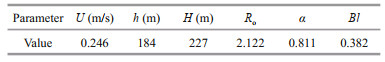
Many characteristic parameters, including Rossby number (Ro=U/fL), fractional height of seamounts (α=h/H) and blocking factor (Bl=α/Ro), have been proposed to determine whether a Taylor cap can form in a seamount. U is the average velocity of the impinging flow, f is the Coriolis parameter, L is the horizontal length of the seamount, H is the fluid depth, and h is the height of the seamount within the range of the impacting flow (Hogg, 1973; Owens and Hogg, 1980; Chapman and Haidvogel, 1992; White et al., 2007).
The calculation parameters in M4 seamount is shown in Fig. 11, and the environmental conditions and calculation results are given in Table 1. The threshold values for Taylor cap formation may vary slightly in different works. The threshold value of Bl was 1 in some studies (Huppert, 1975; Roden, 1987; Martin and Drucker, 1997). Chapman and Haidvogel (1992) and Hogg (1973) proposed that the threshold value of Bl is 4, and the Taylor cap would form under a condition Bl>4. Meanwhile, Chapman and Haidvogel (1992) also put forward that the threshold value of Ro was 0.2, above which the Taylor cap would not form. The calculation results show that values of Bl and Ro are 0.382 and 2.122 in M4 seamount, which do not meet the threshold values to form a Taylor cap mentioned above. Moreover, the Taylor cap is not the main physical process in seamount because it only exists when the current is unidirectional and steady (Beckmann and Mohn, 2002; Lavelle and Mohn, 2010).

|
| Fig.11 The calculation parameters in Section B of M4 seamount Detailed bathymetry data comes from Gan et al. (2021). |
Previous studies have shown that in many cases, the anticyclonic circulation around seamount is mainly caused by the tides (Eriksen, 1991; Kunze and Toole, 1997). Instead, there are few cases of anticyclone circulation caused by mean flow impinging the seamounts. The tidal current over the seamount can generate the residual mean current, and this is commonly referred as "tidal rectification". Tidal rectification is a result of tidal current interacting with the steep bathymetry, then an asymmetry in tidal transport generated by a combined effect of bottom friction and topographic acceleration. Finally, a cold dome forms over the seamount, which is particularly like the uplifted isotherms formed by a Taylor cap (Lavelle and Mohn, 2010).
The reason why the cold dome above the seamount can be maintained is probably that a secondary circulation may also be generated over the seamount (Eriksen, 1991; Brink, 1995). The secondary circulation consists of the vertical flow above the summit and the radial outflow at the edge of the seamount (Fig. 12). Upwelling is generated at the outer border of the anticyclonic circulation, with inward flow above it (Haidvogel et al., 1993), thus forming a closed system. Fundamentally speaking, this circulation system results from the complex balance of the turbulent mixing processes (Haidvogel et al., 1993; Brink, 1995; Kunze and Toole, 1997). The distributions of potential density, temperature, and salinity near the summit of M4 seamount are highly consistent with the closed circulation system caused by tidal rectification (Figs. 10 & 12). The dome-like deformation of isolines in both Section A and Section B corresponds to the cold dome caused by tidal rectification. The uplifted isolines at the edge of the summit are consistent with the upwelling at the outer border of the anticyclonic circulation. Moreover, the vertical flow above the summit may cause the depression of the isolines in the similar position. Therefore, we tend to believe that the tidal current is the main dynamic process controlling the formation of cold dome over M4 seamount.

|
| Fig.12 The anticyclonic circulation and secondary circulation generated around the seamount (based on White et al., 2007) The fork and dot indicate opposite flow directions. |
Turbulent mixing plays a very important role in controlling the physical properties of seawater and affecting the transport of nutrients and the concentration of particles. Early studies have shown that the turbulent diffusivity is only 10-6–10-5 m2/s in the ocean far away from the coastline (Gregg, 1987; Ledwell et al., 1993; Kunze and Sanford, 1996). However, Munk (1966) pointed out as early as 1966 that the average turbulent diffusivity of the global ocean needed to up to at least 10-4 m2/s to maintain the stability of the stratification structure. Therefore, many scholars focused on the boundaries, ridges, channels, and seamounts, and confirmed that these areas did have strong mixing through field measurements. The turbulent diffusivity in these areas is 10–104 times of that in the open ocean (Lueck and Mudge, 1997; Ferron et al., 1998; Lavelle et al., 2004; Ding et al., 2017), thus the global average turbulent diffusivity is still likely to up to 10-4 m2/s. As stated, these special areas have an important impact on the vertical mixing and the transport of heat and materials in the global ocean.
The turbulent diffusivities (K) in M4 seamount are calculated from temperature data (noise is 0.001 ℃) using the Thorpe method (Ferron et al., 1998). The Thorpe scale that can be resolved depends on the sampling rate and noise level of the instrument. In this work, we use CTD data that were previously filtered and subsampled to 1 m to attenuate high-frequency noise. Hence, we cannot resolve gravitational overturns smaller than 2 m or Thorpe scales less than 1 m. The use of a CTD data is sufficient to resolve the main instabilities, but Thorpe scale of 0 does not necessarily imply that there is no overturn. The profiles of all 21 stations are shown in Figs. 13 & 14. The high K values in M4 seamount mostly distribute in the surface layer, ~500 m and near the bottom, with the magnitude of 10-3–10-1 m2/s (Figs. 13b & 14b).

|
| Fig.13 The profiles of the turbulent diffusivities (K) in Section A of M4 seamount a. upper 300 m of Section A; b. full depth of Section A. |

|
| Fig.14 The profiles of the turbulent diffusivities (K) in Section B of M4 seamount a. upper 300 m of Section B; b. full depth of Section B. |
Although the thermocline in M4 seamount is deep enough in summer, but the high K values are only distributed in very shallow water layer due to the strong stratification. But there is still difference in the depth distribution of surface K (we refer it as "surface turbulent layer") at different stations (Figs. 13a & 14a). Previous studies have shown that there is a certain correlation between turbulence and tidal phase (Muench et al., 2009; Padman et al., 2009), that is, higher tidal velocity will have a greater impact on the turbulent diffusivity K. We analyze the correlation between the thickness of surface turbulent layer and the four main tidal constituents of M4 seamount during the survey time (Fig. 15). The results show that there are some connections between the thickness of surface turbulent layer and the constituents M2, S2, and O1, while the correlation between the thickness and diurnal constituent K1 is poor. Nevertheless, the tidal phase does have an effect on turbulence anyway. The influence of semidiurnal constituents on the surface turbulence in M4 seamount is more significant than that of diurnal constituents. The larger the tidal velocity is, the thicker the surface turbulent layer is, and the deeper the water can be affected.

|
| Fig.15 Correlations between the thickness of surface turbulent layer and four main tidal constituents of M4 seamount |
The turbulent diffusivity at the surface layer is always affected by the surface wind stress. Figure 16 shows the monthly mean wind field at 10 m above the sea surface around M4 seamount in August 2017. The wind speed around M4 seamount in August 2017 is relatively small, ranges 1–4 m/s. The theoretical calculation (Wang et al., 2006) result of the surface wind stress around M4 seamount is ~0.020 N/m2. The magnitude of the turbulent diffusivity caused by surface wind stress is approximately 10-5.3 m2/s (Jing and Wu, 2010). It is obviously that the surface wind stress has little effect on the turbulent mixing of M4 seamount.

|
| Fig.16 The monthly mean wind field at 10 m above the sea surface around M4 seamount in August 2017 The monthly mean wind data were accessed from the NCEP Reanalysis data provided by the NOAA/OAR/ESRL PSL, Boulder, Colorado, USA, from https://psl.noaa.gov/. The black triangle represents M4 seamount. |
In addition to surface wind stress, the effect of the eddy is also considered. Seamounts are known to be places of ocean eddies creation and destruction (Royer, 1978; Herbette et al., 2003), and as a result, eddies are bound to have an impact on the hydrodynamics of seamounts.
Figure 17 shows the characteristics of SSHA in the study area in August 2017. Almost the whole study area presents a positive SSHA with the maximum value of +0.3 m, and the activities of these warm eddies are energetic. There is a large warm eddy in the east of M4 seamount on August 15, and it moves westward with time and breaks into several small eddies when passing through the seamount. Observation and hydrodynamic models suggest that during interaction with a seamount, an eddy may disintegrate over the seamount, split into two or just be rotated around the seamount flank as it passes by. However, even in the latter case, the eddy may transfer its own water and energy to the seamount system when it survives the collision (Richardson et al., 2000; Adduce and Cenedese, 2004). The energy can be used to induce turbulent mixing in the seamount. Therefore, the high surface turbulent diffusivities in M4 seamount may be partly related to the vigorous activities of warm eddies. However, the near-surface turbulent diffusivities do not decay to small background levels at stations far from the seamount, and the near-surface salinity is strongly stratified (Fig. 10) in the presence of such strong mixing. There may be other factors that need to be studied further.

|
| Fig.17 SSHA around M4 seamount during the survey time a. August 15; b. August 20; c. August 25; d. August 30. The black triangle represents M4 seamount. |
There are also high turbulent diffusivities near 500 m in the water column (Figs. 13b & 14b). Two explanations are possible for this phenomenon. One is that the warm eddies mentioned above may disturb the underlying thermocline and create velocity anomalies at depth. And the eddy-related mixing may also reach to around 500-m depth. Besides, the mixing of NPIW from the north and AAIW from the south occurs near the depth of 500 m. There may be a strong density front between these two water masses and the interaction of strong frontal currents with topography is a probable cause of elevated mixing (Park et al., 2014). These two explanations need further confirmations.
The turbulent diffusivities near the bottom of most stations in M4 seamount show high values (Figs. 13b & 14b). However, there is no high turbulent diffusivity near the bottom of stations B-5, B-6, B-10, and B-11 which are far away from the seamount (Fig. 14b). According to previous studies, the interaction of steep bathymetry and semidiurnal tides will produce the most energetic internal tides in the ocean, and as a result, the intensity of internal tides above the summit and slopes of a seamount is relatively high (Munk, 1981; Lavelle and Mohn, 2010). The energy will be redistributed by the breaking of fragile internal tides, which leads to vigorous turbulent mixing (Rudnick et al., 2003; van Haren and Gostiaux, 2012). This mechanism is in good agreement with the distribution of turbulent diffusivities in M4 seamount. The turbulent diffusivities near the bottom of most stations at steep slope show high values and stations located at flat terrain have no high turbulent diffusivity near the bottom (Figs. 13b & 14b). Hence, the tidal/topography interaction is the plausible cause of the mixing at the bottom of M4 seamount. In addition, the interaction between the bottom current and topography may also cause the high turbulent diffusivities near the bottom of M4 seamount and measurement current data near the bottom are necessary to confirm this hypothesis.
As the above, the surface wind stress, tidal phase, especially the interaction between M4 seamount and all kinds of current and mesoscale eddies all could be important factors affecting the distribution of turbulent diffusivity in M4 seamount. Strong mixing was also found on other steep terrains. Lueck and Mudge (1997) estimated the rate of dissipation of kinetic energy around Cobb Seamount and showed that mixing there is 100 to 10 000 times as large as that far away from the seamount. They thought the internal waves were a likely source of energy for the strong turbulence around Cobb Seamount. Large turbulent diffusivities also occurred in other steep terrains like fracture zones in the ocean. The turbulent diffusivity in the Romanche Fracture Zone was measured by Ferron et al. (1998). A mean turbulent diffusivity of about 0.1 m2/s was found for the bottom water in this region and the mixing was a major component of the heat flux transfers between deep and bottom water masses, and exerts a significant control on the thermohaline circulation equilibrium.
5 CONCLUSIONThe upper 200 m of water in M4 seamount is controlled by NEC, and the direction of the current in this layer is westward with a relatively large velocity of 0.10–0.35 m/s. The water between 300–1 000 m is controlled by NEUC. The current direction is eastward in most stations at a lower velocity of 0.05–0.20 m/s. M4 seamount plays an important role in the current distribution. The current direction at the upstream stations fluctuates greatly below 300 m, and the current direction below 300 m of station at the lee side changes with the distance from seamount. These are likely caused by the obstacle of M4 seamount to NEUC or related to temporal variations.
The water is intensively stratified in the upper 300 m at M4 seamount, and both the thermocline and halocline locate at 100–200 m. NPTW is distributed in the subsurface layer of M4 seamount, and the mixing of NPIW and AAIW in the middle layer results in the uneven distribution of salinity.
The calculation results show that the cold dome above M4 seamount is not caused by a Taylor cap. Tidal currents in M4 seamount are squeezed by the topography and amplified. The interaction between the amplified tidal current and the seamount results in an anticyclone circulation over the seamount, which leads to a cold dome above the summit. In addition, the secondary circulation generates an upwelling at the outer border of the anticyclone eddy and an inward flow above it, forming a closed circulation system. The combination of anticyclone circulation and secondary circulation generates strong uplift of the isolines at the edge of the summit and over the summit in Section B. Moreover, the isolines are depressed between the uplifted contour lines and the bottom of the summit.
The high turbulent diffusivities in M4 seamount are mostly distributed in the surface, ~500 m and near bottom layers, with the magnitude of 10-3–10-1 m2/s. In the surface layer, the tidal phase has an effect on the thickness of the turbulent layer, i.e., the faster the tidal velocity is, the thicker the corresponding surface turbulent layer is, and the deeper the water depth can be affected. In addition, the influence of semidiurnal constituents is greater than that of diurnal constituents. The turbulent diffusivities in the surface of M4 seamount are much larger than that in the open ocean. A calculation result shows that the surface wind stress has little effect on the turbulent mixing of M4 seamount, but the high surface turbulent diffusivities may be partly related to the vigorous activities of warm eddies. The high turbulent diffusivities near the depth of 500 m could be caused by warm eddies around M4 seamount or the interaction of a strong density frontal current between NPIW and AAIW with topography. Near the bottom of M4 seamount, the interaction of steep bathymetry and semidiurnal tides is the most likely cause inducing internal tides, which then lead to the turbulent mixing and furthermore result in the high turbulent diffusivities in most stations, while other stations far away from the seamount only have a background turbulent diffusivity. Additionally, the interaction between the bottom current and topography may also cause the high turbulent diffusivities near the bottom.
6 DATA AVAILABILITY STATEMENTThe site investigation data that support the findings of this study are available from the corresponding author on reasonable request. Links to all the opensource data have been given in the manuscript.
7 ACKNOWLEDGMENTThe authors would like to thank the crew and scientists aboard R/V Kexue from the Institute of Oceanology, Chinese Academy of Sciences for their support and help to the investigation of this study. The authors gratefully thank the reviewers for their insightful comments.
Adduce C, Cenedese C. 2004. An experimental study of a mesoscale vortex colliding with topography of varying geometry in a rotating fluid. Journal of Marine Research, 62(5): 611-638.
DOI:10.1357/0022240042387583 |
Beckmann A, Mohn C. 2002. The upper ocean circulation at Great Meteor Seamount. Ocean Dynamics, 52(4): 194-204.
DOI:10.1007/s10236-002-0018-3 |
Brink K H. 1995. Tidal and lower frequency currents above Fieberling Guyot. Journal of Geophysical Research: Oceans, 100(C6): 10 817-10 832.
DOI:10.1029/95JC00998 |
Chapman D C, Haidvogel D B. 1992. Formation of Taylor Caps over a tall isolated seamount in a stratified ocean. Geophysical & Astrophysical Fluid Dynamics, 64(1-4): 31-65.
DOI:10.1080/03091929208228084 |
Chassignet E P, Hurlburt H E, Smedstad O M, Halliwell G R, Hogan P J, Wallcraft A J, Bleck R. 2006. Ocean prediction with the hybrid coordinate ocean model (HYCOM). In: Chassignet E P, Verron J eds. Ocean Weather Forecasting: An Integrated View of Oceanography. Springer, Dordrecht. p. 413-426.
|
Clark M R, Rowden A A, Schlacher T, Williams A, Consalvey M, Stocks K I, Rogers A D, O'Hara T D, White M, Shank T M, Hall-Spencer J M. 2010. The ecology of seamounts: structure, function, and human impacts. Annual Review of Marine Science, 2: 253-278.
DOI:10.1146/annurev-marine-120308-081109 |
Ding W X, Liang C J, Liao G H, Gao L B. 2017. The turbulent diffusivity estimation in Prydz Bay, Antarctic. Journal of Marine Sciences, 35(1): 14-24.
(in Chinese with English abstract) DOI:10.3969/j.issn.1001-909X.2017.01.002 |
Egbert G D, Erofeeva S Y. 2002. Efficient inverse modeling of Barotropic ocean tides. Journal of Atmospheric and Oceanic Technology, 19(2): 183-204.
DOI:10.1175/1520-0426(2002)019<0183:EIMOBO>2.0.CO;2 |
Eriksen C C. 1991. Observations of amplified flows atop a large seamount. Journal of Geophysical Research: Oceans, 96(C8): 15 227-15 236.
DOI:10.1029/91jc01176 |
Ferron B, Mercier H, Speer K, Gargett A, Polzin K. 1998. Mixing in the Romanche fracture zone. Journal of Physical Oceanography, 28(10): 1 929-1 945.
DOI:10.1175/1520-0485(1998)028<1929:mitrfz>2.0.co;2 |
Gan Y, Ma X C, Luan Z D, Yan J. 2021. Morphology and multifractal features of a guyot in specific topographic vicinity in the Caroline Ridge, West Pacific. Journal of Oceanology and Limnology, 39(5): 1 591-1 604.
DOI:10.1007/s00343-021-0383-8 |
Genin A, Dayton P K, Lonsdale P F, Spiess F N. 1986. Corals on seamount peaks provide evidence of current acceleration over deep-sea topography. Nature, 322(6074): 59-61.
DOI:10.1038/322059a0 |
Genin A. 2004. Bio-physical coupling in the formation of zooplankton and fish aggregations over abrupt topographies. Journal of Marine Systems, 50(1-2): 3-20.
DOI:10.1016/j.jmarsys.2003.10.008 |
Gregg M C. 1987. Diapycnal mixing in the thermocline: a review. Journal of Geophysical Research: Oceans, 92(C5): 5 249-5 286.
DOI:10.1029/JC092iC05p05249 |
Haidvogel D B, Beckmann A, Chapman D C, Lin R Q. 1993. Numerical simulation of flow around a tall isolated seamount. Part Ⅱ: resonant generation of trapped waves. Journal of Physical Oceanography, 23(11): 2 373-2 391.
DOI:10.1175/1520-0485(1993)023<2373:NSOFAA>2.0.CO;2 |
Herbette S, Morel Y, Arhan M. 2003. Erosion of a surface vortex by a seamount. Journal of Physical Oceanography, 33(8): 1 664-1 679.
DOI:10.1175/2382.1 |
Hogg N G. 1973. On the stratified Taylor column. Journal of Fluid Mechanics, 58(3): 517-537.
DOI:10.1017/S0022112073002302 |
Hu D X, Wu L X, Cai W J, Gupta A S, Ganachaud A, Qiu B, Gordon A L, Lin X P, Chen Z H, Hu S J, Wang G J, Wang Q Y, Sprintall J, Qu T D, Kashino Y J, Wang F, Kessler W S. 2015. Pacific western boundary currents and their roles in climate. Nature, 522(7556): 299-308.
DOI:10.1038/nature14504 |
Huppert H E. 1975. Some remarks on the initiation of inertial Taylor columns. Journal of Fluid Mechanics, 67(2): 397-412.
DOI:10.1017/S0022112075000377 |
Jing Z, Wu L X. 2010. Seasonal variation of turbulent diapycnal mixing in the northwestern Pacific stirred by wind stress. Geophysical Research Letters, 37(23): L23604.
DOI:10.1029/2010GL045418 |
Kunze E, Sanford T B. 1996. Abyssal mixing: where it is not. Journal of Physical Oceanography, 26(10): 2 286-2 296.
DOI:10.1175/1520-0485(1996)026<2286:AMWIIN>2.0.CO;2 |
Kunze E, Toole J M. 1997. Tidally driven vorticity, diurnal shear, and turbulence atop fieberling seamount. Journal of Physical Oceanography, 27(12): 2 663-2 693.
DOI:10.1175/1520-0485(1997)027<2663:TDVDSA>2.0.CO;2 |
Lavelle J W, Lozovatsky I D, Smith IV D C. 2004. Tidally induced turbulent mixing at Irving Seamount-modeling and measurements. Geophysical Research Letters, 31(10): L10308.
DOI:10.1029/2004GL019706 |
Lavelle J W, Mohn C. 2010. Motion, commotion, and biophysical connections at deep ocean seamounts. Oceanography, 23(1): 90-103.
DOI:10.5670/oceanog.2010.64 |
Ledwell J R, Watson A J, Law C S. 1993. Evidence for slow mixing across the pycnocline from an open-ocean tracerrelease experiment. Nature, 364(6439): 701-703.
DOI:10.1038/364701a0 |
Li F Q, Su Y S. 2000. Analysis of Water Masses in Oceans. Qingdao Ocean University Press, Qingdao, China: 397p.
(in Chinese) |
Lueck R G, Mudge T D. 1997. Topographically induced mixing around a shallow seamount. Science, 276(5320): 1 831-1 833.
DOI:10.1126/science.276.5320.1831 |
Martin S, Drucker R. 1997. The effect of possible Taylor columns on the summer ice retreat in the Chukchi Sea. Journal of Geophysical Research: Oceans, 102(C5): 10 473-10 482.
DOI:10.1029/97jc00145 |
Masumoto Y, Yamagata T. 1991. Response of the Western Tropical Pacific to the Asian Winter Monsoon: The Generation of the Mindanao Dome. Journal of Physical Oceanography, 21(9): 1 386-1 398.
DOI:10.1175/1520-0485(1991)021<1386:ROTWTP>2.0.CO;2 |
Mohn C, Beckmann A. 2002. The upper ocean circulation at great meteor seamount. Ocean Dynamics, 52(4): 179-193.
DOI:10.1007/s10236-002-0017-4 |
Muench R, Padman L, Gordon A, Orsi A. 2009. A dense water outflow from the Ross Sea, Antarctica: mixing and the contribution of tides. Journal of Marine Systems, 77(4): 369-387.
DOI:10.1016/j.jmarsys.2008.11.003 |
Munk W H. 1966. Abyssal recipes. Deep Sea Research and Oceanographic Abstracts, 13(4): 707-730.
DOI:10.1016/0011-7471(66)90602-4 |
Munk W H. 1981. Internal waves and small scale processes. In: Warren B, Wunch C eds. Evolution of Physical Oceanography. MIT Press, Cambridge. p. 264-276.
|
Owens W B, Hogg N G. 1980. Oceanic observations of stratified Taylor columns near a bump. Deep Sea Research Part A. Oceanographic Research Papers, 27(12): 1 029-1 045.
DOI:10.1016/0198-0149(80)90063-1 |
Padman L, Howard S L, Orsi A H, Muench R D. 2009. Tides of the northwestern Ross Sea and their impact on dense outflows of Antarctic Bottom Water. Deep Sea Research Part Ⅱ: Topical Studies in Oceanography, 56(13-14): 818-834.
DOI:10.1016/j.dsr2.2008.10.026 |
Park Y H, Lee J H, Durand I, Hong C S. 2014. Validation of Thorpe-scale-derived vertical diffusivities against microstructure measurements in the Kerguelen region. Biogeosciences, 11(23): 6 927-6 937.
DOI:10.5194/bg-11-6927-2014 |
Qiu B, Rudnick D L, Cerovecki I, Cornuelle B D, Chen S M, Schönau M C, McClean J L, Gopalakrishnan G. 2015. The Pacific North Equatorial Current: new insights from the origins of the Kuroshio and Mindanao Currents(OKMC) project. Oceanography, 28(4): 24-33.
DOI:10.5670/oceanog.2015.78 |
Read J, Pollard R. 2017. An introduction to the physical oceanography of six seamounts in the southwest Indian Ocean. Deep Sea Research Part Ⅱ: Topical Studies in Oceanography, 136: 44-58.
DOI:10.1016/j.dsr2.2015.06.022 |
Richardson P L, Bower A S, Zenk W. 2000. A census of meddies tracked by floats. Progress in Oceanography, 45(2): 209-250.
DOI:10.1016/S0079-6611(99)00053-1 |
Roden G I, Taft B A. 1985. Effect of the Emperor Seamounts on the mesoscale thermohaline structure during the summer of 1982. Journal of Geophysical Research: Oceans, 90(C1): 839-855.
DOI:10.1029/JC090iC01p00839 |
Roden G I. 1987. Effect of seamounts and seamount chains on ocean circulation and thermohaline structure. In: Keating B H, Fryer P, Batiza R, Boehlert G W eds. Seamounts, Islands, and Atolls. American Geophysical Union, Washington. p. 335-354, https://doi.org/10.1029/GM043p0335.
|
Rogers A D. 1994. The biology of seamounts. Advances in Marine Biology, 30: 305-350.
DOI:10.1016/S0065-2881(08)60065-6 |
Rowden A A, Dower J F, Schlacher T A, Consalvey M, Clark M R. 2010. Paradigms in seamount ecology: fact, fiction and future. Marine Ecology, 31(s1): 226-241.
DOI:10.1111/j.1439-0485.2010.00400.x |
Royer T C. 1978. Ocean eddies generated by seamounts in the North Pacific. Science, 199(4333): 1 063-1 064.
DOI:10.1126/science.199.4333.1063-a |
Rudnick D L, Boyd T J, Brainard R E, Carter G S, Egbert G D, Gregg M C, Holloway P E, Klymak J M, Kunze E, Lee C M, Levine M D, Luther D S, Martin J P, Merrifield M A, Moum J N, Nash J D, Pinkel R, Rainville L, Sanford T B. 2003. From tides to mixing along the Hawaiian Ridge. Science, 301(5631): 355-357.
DOI:10.1126/science.1085837 |
Shank T M. 2010. Seamounts: deep-ocean laboratories of faunal connectivity, evolution, and endemism. Oceanography, 23(1): 108-122.
DOI:10.5670/oceanog.2010.65 |
United States Board on Geographic Names. 1981. Gazetteer of Undersea Features: Names Approved by the United States Board on Geographic Names. Defense Mapping Agency, Washington.
|
van Haren H, Gostiaux L. 2012. Detailed internal wave mixing above a deep-ocean slope. Journal of Marine Research, 70(1): 173-197.
DOI:10.1357/002224012800502363 |
Vianello P, Ternon J F, Demarcq H, Herbette S, Roberts M J. 2020. Ocean currents and gradients of surface layer properties in the vicinity of the Madagascar Ridge(including seamounts) in the South West Indian Ocean. Deep Sea Research Part Ⅱ: Topical Studies in Oceanography, 176: 104816.
DOI:10.1016/j.dsr2.2020.104816 |
Wang F, Zang N, Li Y L, Hu D X. 2015. On the subsurface countercurrents in the Philippine Sea. Journal of Geophysical Research: Oceans, 120(1): 131-144.
DOI:10.1002/2013JC009690 |
Wang G H, Chen D K, Su J L. 2006. Generation and life cycle of the dipole in the South China Sea summer circulation. Journal of Geophysical Research: Oceans, 111(C6): C06002.
DOI:10.1029/2005JC003314 |
White M, Bashmachnikov I, Arístegui J, Martins A. 2007. Physical processes and seamount productivity. In: Pitcher T J, Morato T, Hart P J B, Clark M R, Haggan N, Santos R S eds. Seamounts: Ecology, Fisheries & Conservation. Blackwell Publishing, Hoboken. p. 65-84, https://doi.org/10.1002/9780470691953.ch4.
|
Xie L L, Tian J W, Hu D X, Wang F. 2009. A quasi-synoptic interpretation of water mass distribution and circulation in the western North Pacific: I. water mass distribution. Chinese Journal of Oceanology and Limnology, 27(3): 630-639.
DOI:10.1007/s00343-009-9161-8 |
Zhang J L, Xu K D. 2013. Progress and prospects in seamount biodiversity. Advances in Earth Science, 28(11): 1 209-1 216.
(in Chinese with English abstract) |
Zhang L L, Wang F J, Wang Q Y, Hu S J, Wang F, Hu D X. 2017. Structure and variability of the north equatorial current/undercurrent from mooring measurements at 130°E in the western Pacific. Scientific Reports, 7(1): 46 310.
DOI:10.1038/srep46310 |
Zhang Q L, Zhou H, Liu H W. 2012. Interannual variability in the Mindanao eddy and its impact on thermohaline structure pattern. Acta Oceanologica Sinica, 31(6): 56-65.
DOI:10.1007/s13131-012-0247-3 |